B.4 Interior-Point Methods
Traditional optimization algorithms based on gradient projection methods may suffer from slow convergence and sensitivity to the algorithm initialization and stepsize selection. The more modern interior-point methods (IPM) for convex problems enjoy excellent convergence properties (polynomial convergence) and do not suffer from the usual problems of the traditional methods. Some standard textbooks that cover IPMs in detail include Nesterov and Nemirovski (1994), Ye (1997), Nesterov (2018), Bertsekas (1999), Nemirovski (2000), Ben-Tal and Nemirovski (2001), Boyd and Vandenberghe (2004), Luenberger and Ye (2021), and Nocedal and Wright (2006).
Consider the following convex optimization problem: \[\begin{equation} \begin{array}{ll} \underset{\bm{x}}{\textm{minimize}} & \begin{array}[t]{l} f_0(\bm{x}) \end{array}\\ \textm{subject to} & \begin{array}[t]{l} f_i(\bm{x}) \leq 0, \qquad i=1,\dots,m,\\ \bm{A}\bm{x} = \bm{b}, \end{array} \end{array} \tag{B.2} \end{equation}\] where all \(f_i\) are convex and twice continuously differentiable, and \(\bm{A}\in\R^{p\times n}\) is a fat (i.e., more columns than rows), full rank matrix. We assume that the optimal value \(p^\star\) is finite and attained, and that the problem is strictly feasible, hence strong duality holds and dual optimum is attained.
B.4.1 Eliminating Equality Constraints
Equality constraints can be conveniently dealt with via Lagrange duality (Boyd and Vandenberghe, 2004). Alternatively, they can be simply eliminated in a pre-processing stage as shown next.
From linear algebra, we know that the possibly infinite solutions to \(\bm{A}\bm{x} = \bm{b}\) can be represented as follows: \[ \{\bm{x} \in \R^n \mid \bm{A}\bm{x} = \bm{b}\} = \{\bm{F}\bm{z} + \bm{x}_0 \mid \bm{z} \in \R^{n-p}\}, \] where \(\bm{x}_0\) is any particular solution to \(\bm{A}\bm{x} = \bm{b}\) and the range of \(\bm{F} \in \R^{n\times(n-p)}\) is the nullspace of \(\bm{A}\in\R^{p\times n}\), that is, \(\bm{A}\bm{F} = \bm{0}\).
The reduced or eliminated problem equivalent to problem (B.2) is \[ \begin{array}{ll} \underset{\bm{z}}{\textm{minimize}} & \tilde{f}_0(\bm{z}) \triangleq f_0(\bm{F}\bm{z} + \bm{x}_0)\\ \textm{subject to} & \tilde{f}_i(\bm{z}) \triangleq f_i(\bm{F}\bm{z} + \bm{x}_0) \leq 0, \qquad i=1,\dots,m, \end{array} \] where each function \(\tilde{f}_i\) has gradient and Hessian given by \[ \begin{aligned} \nabla \tilde{f}_i(\bm{z}) &= \bm{F}^\T \nabla f_i(\bm{x}),\\ \nabla^2 \tilde{f}_i(\bm{z}) &= \bm{F}^\T \nabla^2 f_i(\bm{x}) \bm{F}. \end{aligned} \]
Once the solution \(\bm{z}^\star\) to the reduced problem has been obtained, the solution to the original problem (B.2) can be readily derived as \[ \bm{x}^\star = \bm{F}\bm{z}^\star + \bm{x}_0. \]
B.4.2 Indicator Function
We can equivalently reformulate problem (B.2) via the indicator function as \[ \begin{array}{ll} \underset{\bm{x}}{\textm{minimize}} & f_0(\bm{x}) + \sum_{i=1}^m I_{-}\left(f_i(\bm{x})\right)\\ \textm{subject to} & \bm{A}\bm{x} = \bm{b}, \end{array} \] where the indicator function is defined as \[ I_{-}(u) = \begin{cases} 0 & \textm{if }u\le0,\\ \infty & \textm{otherwise}. \end{cases} \] In this form, the inequality constraints have been eliminated at the expense of the indicator function in the objective. Unfortunately, the indicator function is a noncontinuous, nondifferentiable function, which is not practical.
B.4.3 Logarithmic Barrier
In practice, we need to use some smooth approximation of the indicator function. A very popular and convenient choice is the so-called logarithmic barrier: \[ I_{-}(u) \approx -\frac{1}{t}\textm{log}(-u), \] where \(t>0\) is a parameter that controls the approximation and improves as \(t \rightarrow \infty\). Figure B.1 illustrates the logarithmic barrier for several values of \(t\).
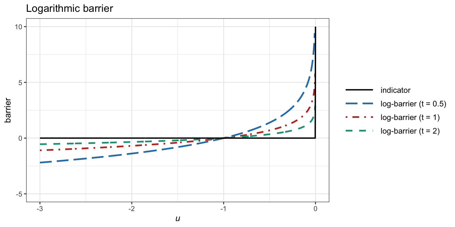
Figure B.1: Logarithmic barrier for several values of the parameter \(t\).
With the logarithmic barrier, we can approximate the problem (B.2) as \[ \begin{array}{ll} \underset{\bm{x}}{\textm{minimize}} & f_0(\bm{x}) -\frac{1}{t}\sum_{i=1}^m \textm{log}\left(-f_i(\bm{x})\right)\\ \textm{subject to} & \bm{A}\bm{x} = \bm{b}. \end{array} \]
We can define the overall logarithmic barrier function (excluding the \(1/t\) factor) as \[ \phi(\bm{x}) = -\sum_{i=1}^m \textm{log}\left(-f_i(\bm{x})\right), \] which is convex (from the composition rules in Section A.3) with gradient and Hessian given by \[ \begin{aligned} \nabla \phi(\bm{x}) &= \sum_{i=1}^m\frac{1}{-f_i(\bm{x})}\nabla f_i(\bm{x}),\\ \nabla^2 \phi(\bm{x}) &= \sum_{i=1}^m\frac{1}{f_i(\bm{x})^2}\nabla f_i(\bm{x}) \nabla f_i(\bm{x})^\T + \sum_{i=1}^m\frac{1}{-f_i(\bm{x})}\nabla^2 f_i(\bm{x}). \end{aligned} \]
B.4.4 Central Path
For convenience, we multiply the objective function by a positive scalar \(t > 0\) and define \(\bm{x}^\star(t)\) as the solution to the equivalent problem \[\begin{equation} \begin{array}{ll} \underset{\bm{x}}{\textm{minimize}} & t f_0(\bm{x}) + \phi(\bm{x})\\ \textm{subject to} & \bm{A}\bm{x} = \bm{b}, \end{array} \tag{B.3} \end{equation}\] which can be conveniently solved via Newton’s method.
The central path is defined as the curve \(\{\bm{x}^\star(t) \mid t>0\}\) (assuming that the solution for each \(t\) is unique). Figure B.2 illustrates the central path of an LP.

Figure B.2: Example of central path of an LP.
Ignoring the equality constraints for convenience of exposition, a solution to (B.3), \(\bm{x}^\star(t)\), must satisfy the equation \[ t\nabla f_0(\bm{x}) + \sum_{i=1}^m\frac{1}{-f_i(\bm{x})}\nabla f_i(\bm{x}) = \bm{0}. \] Equivalently, defining \(\lambda_i^\star(t) = 1/(-tf_i(\bm{x}^\star(t)))\), the point \(\bm{x}^\star(t)\) minimizes the Lagrangian \[ L(\bm{x};\bm{\lambda}^\star(t)) = f_0(\bm{x}) + \sum_{i=1}^m \lambda_i^\star(t)f_i(\bm{x}). \] This confirms the intuitive idea that \(f_0(\bm{x}^\star(t)) \rightarrow p^\star\) as \(t\rightarrow\infty\). In particular, from Lagrange duality theory (refer to Section A.6.3 in Appendix A for details), \[ \begin{aligned} p^\star &\ge g\left(\bm{\lambda}^\star(t)\right)\\ &= L\left(\bm{x}^\star(t);\bm{\lambda}^\star(t)\right)\\ &= f_0\left(\bm{x}^\star(t)\right) - m/t. \end{aligned} \]
In addition, the central path has a nice connection with the Karush–Kuhn–Tucker (KKT) optimality conditions (refer to Section A.6.4 for details). In particular, the point \(\bm{x}^\star(t)\) together with the dual point \(\bm{\lambda}^\star(t)\) satisfy the following: \[ \begin{array}{rl} f_{i}(\bm{x}) \leq0,\quad i=1,\dots,m, & \quad \textm{(primal feasibility)}\\ \lambda_{i} \ge0,\quad i=1,\dots,m, & \quad \textm{(dual feasibility)}\\ \qquad\qquad\qquad\lambda_{i}f_{i}(\bm{x}) = -\frac{1}{t},\quad i=1,\dots,m, & \quad \textm{(approximate complementary slackness)}\\ \nabla f_{0}(\bm{x}) + \sum\limits_{i=1}^{m}\lambda_{i}\nabla f_{i}(\bm{x}) = \bm{0}. & \quad \textm{(zero Lagrangian gradient)}\\ \end{array} \] Clearly, the difference from the KKT conditions of the original constrained problem (see (A.23) in Appendix A) is that the complementary slackness is now approximately satisfied, with the approximation becoming better as \(t\rightarrow\infty\).
B.4.5 Barrier Method
Problem (B.3) with the logarithmic barrier is a smooth approximation of the original constrained problem (B.2), and the approximation gets better as \(t\rightarrow\infty\).
One might be tempted to choose a very large value for \(t\) and then apply Newton’s method to solve the problem. However, this approach would lead to very slow convergence because the gradients and Hessians would experience extremely large variations near the boundary of the feasible set. Consequently, the convergence of Newton’s method would be hindered, failing to reach the phase of quadratic convergence. On the other hand, a small value of \(t\) would facilitate better convergence, but the resulting approximation would not be satisfactorily close to the original problem.
Instead of directly choosing one value for \(t\), we may change it over the iterations in an appropriate way, in order to achieve the best of both worlds: fast convergence and an accurate approximation to the original problem. More specifically, at each outer iteration, the value of \(t\) is updated and then the solution \(\bm{x}^\star(t)\) is computed (the so-called centering step) with Newton’s method starting at the current point \(\bm{x}\) and running over a few inner iterations. Interior-point methods achieve precisely such a trade-off and they get their name because for each value of \(t>0\) the solution \(\bm{x}^\star(t)\) is strictly feasible and lies in the interior of the feasible set.
The barrier method, which is one type of primal-based IPM, uses a simple, yet effective, way to update the value of \(t\) with the iterations as \(t^{k+1} \gets \mu t^{k}\), where \(\mu>1\) is a parameter and typically \(t^{0}=1\). The choice of \(\mu\) involves a trade-off: large \(\mu\) means fewer outer iterations, but more inner (Newton) iterations; typical values are \(\mu = 10\) to around \(20\). In addition, the termination criterion can be chosen as \(m/t < \epsilon\), guaranteeing \(f_0(\bm{x}) - p^\star \le \epsilon\). Algorithm B.3 summarizes the implementation of the barrier method; the reader is referred to Boyd and Vandenberghe (2004) for practical discussions on the details.
Algorithm B.3: Barrier method for the constrained problem (B.2).
Choose initial point \(\bm{x}^0\in\mathcal{X}\) stricly feasible, \(t^{0}>0\), \(\mu>1\), and tolerance \(\epsilon>0\);
Set \(k \gets 0\);
repeat
- Centering step: compute next iterate \(\bm{x}^{k+1}\) by solving problem (B.3) with \(t=t^{k}\) and initial point \(\bm{x}^{k}\);
- Increase \(t\): \(\quad t^{k+1} \gets \mu t^{k}\);
- \(k \gets k+1\);
until convergence (i.e., \(m/t < \epsilon\));
Example B.4 (Barrier method for LP) Consider the following LP: \[ \begin{array}{ll} \underset{\bm{x}}{\textm{minimize}} & \bm{c}^\T\bm{x}\\ \textm{subject to} & \bm{A}\bm{x} \leq \bm{b}. \end{array} \]
We employ Algorithm B.3 with different values of \(\mu\) to see the effect of this parameter in the total number of Newton iterations.
Figure B.3 shows the convergence for the case of \(m=100\) inequalities and \(n=50\) variables, with \(\epsilon=10^{-6}\) for the duality gap (the centering problem is solved via Newton’s method). We can verify that the total number of Newton iterations is not very sensitive to the choice of \(\mu\) as long as \(\mu\geq10\).
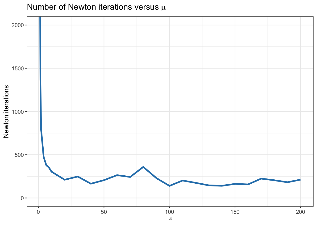
Figure B.3: Convergence of barrier method for an LP for different values of \(\mu\).
B.4.6 Convergence
From the termination criterion in Algorithm B.3, the number of outer iterations (or centering steps) required is \(k\) such that \[ \frac{m}{\mu^k t^0} \leq \epsilon, \] that is, \[ \left\lceil \frac{\textm{log}\left(m/\left(\epsilon t^0\right)\right)}{\textm{log}(\mu)} \right\rceil, \] where \(\lceil \cdot \rceil\) is the ceiling operator. The convergence of each centering step can also be characterized via the convergence for Newton’s method. But this approach ignores the specific updates for \(\mu\) and the good initialization points for each centering step.
For a convergence analysis, the reader is referred to Nesterov and Nemirovski (1994), Nemirovski (2000), Ben-Tal and Nemirovski (2001), Boyd and Vandenberghe (2004), Nesterov (2018), Luenberger and Ye (2021), and Nocedal and Wright (2006).
B.4.7 Feasibility and Phase I Methods
The barrier method in Algorithm B.3 contains a small hidden detail: the need for a strictly feasible initial point \(\bm{x}^{0}\) (such that \(f_i\left(\bm{x}^{0}\right)<0\)). When such a point is not known, the barrier method is preceded by a preliminary stage, called phase I, in which a strictly feasible point is computed. Such a point can then be used as a starting point for the barrier method, which is then called phase II.
There are several phase I methods that can be used to find a feasible point for problem (B.2) by solving the feasibility problem \[ \begin{array}{ll} \underset{\bm{x}}{\textm{find}} & \begin{array}[t]{l} \bm{x} \end{array}\\ \textm{subject to} & \begin{array}[t]{l} f_i(\bm{x}) \leq 0, \qquad i=1,\dots,m,\\ \bm{A}\bm{x} = \bm{b}. \end{array} \end{array} \]
However, note that a barrier method cannot be used to solve the feasibility problem directly because it would also require a feasible starting point.
Phase I methods have to be formulated in a convenient way so that a feasible point can be readily constructed and a barrier method can then be used. A simple example relies on solving the convex optimization problem \[ \begin{array}{ll} \underset{\bm{x},s}{\textm{minimize}} & \begin{array}[t]{l} s \end{array}\\ \textm{subject to} & \begin{array}[t]{l} f_i(\bm{x}) \leq s, \qquad i=1,\dots,m,\\ \bm{A}\bm{x} = \bm{b}. \end{array} \end{array} \] A strictly feasible point can be easily constructed for this problem: choose any value of \(\bm{x}\) that satisfies the equality constraints, and then choose \(s\) satisfying \(s > f_i(\bm{x})\) such as \(s = 1.1 \times \text{max}_i \{f_i(\bm{x})\}.\) With such an initial strictly feasible point, the feasibility problem can be solved, obtaining \(\left(\bm{x}^\star,s^\star\right)\). If \(s^\star<0\), then \(\bm{x}^\star\) is a strictly feasible point that can be used in the barrier method to solve the original problem (B.2). However, if \(s^\star>0\), it means that no feasible point exists and there is no need to even attempt to solve problem (B.2) since it is infeasible.
B.4.8 Primal-Dual Interior-Point Methods
The barrier method described herein is a primal version of an IPM. However, there are more sophisticated primal–dual IPMs that are more efficient than the primal barrier method when high accuracy is needed. They often exhibit superlinear asymptotic convergence.
The idea is to update the primal and dual variables at each iteration; as a consequence, there is no distinction between inner and outer iterations. In addition, they can start at infeasible points, which alleviates the need for phase I methods.