11.6 Vanilla Convex Formulations
Consider the risk budgeting equations \[w_i\left(\bSigma\w\right)_i = b_i \, \w^\T\bSigma\w, \qquad i=1,\ldots,N\] with \(\bm{1}^\T\w=1\) and \(\w \ge \bm{0}\). If we define \(\bm{x}=\w/\sqrt{\w^\T\bSigma\w}\), then we can rewrite them as \(x_i\left(\bSigma\bm{x}\right)_i = b_i\) or, more compactly in vector form, as \[\begin{equation} \bSigma\bm{x} = \bm{b}/\bm{x} \tag{11.3} \end{equation}\] with \(\bm{x} \ge \bm{0},\) from which we can recover the portfolio simply by normalizing \(\bm{x}\) as \(\w = \bm{x}/(\bm{1}^\T\bm{x})\).
Interestingly, the equations in (11.3) can be rewritten in terms of the correlation matrix \(\bm{C} = \bm{D}^{-1/2}\bSigma\bm{D}^{-1/2}\), with \(\bm{D}\) a diagonal matrix containing the variances \(\textm{diag}(\bSigma) = \bm{\sigma}^2\) along the main diagonal, as (Spinu, 2013) \[\begin{equation} \bm{C}\tilde{\bm{x}} = \bm{b}/\tilde{\bm{x}}, \tag{11.4} \end{equation}\] where \(\bm{x} = \tilde{\bm{x}}/\bm{\sigma}\). This has the effect of normalizing the returns with respect to the volatilities of the assets, which can help numerically as will be empirically verified later.
11.6.1 Direct Resolution via Root Finding
The system of nonlinear equations \(\bSigma\bm{x} = \bm{b}/\bm{x}\) can be interpreted as finding the roots of the nonlinear function \[F(\bm{x}) = \bSigma\bm{x} - \bm{b}/\bm{x},\] that is, solving for \[F(\bm{x}) = \bm{0}.\] In practice, this can be done with a general-purpose nonlinear multivariate root finder, available in most programming languages.53
A similar root-finding problem can be formulated in terms of \(\w\) by including the budget constraint \(\bm{1}^\T\w = 1\) explicitly in the nonlinear function (Chaves et al., 2012): \[ F(\w, \lambda) = \left[\begin{array}{c} \bSigma\bm{w} - \lambda\bm{b}/\bm{w}\\ \bm{1}^\T\w - 1 \end{array}\right]. \]
11.6.2 Formulations
A more interesting way to solve the risk budgeting equation in (11.3) is by unveiling the hidden convexity. This can be achieved by realizing that (11.3) precisely corresponds to the optimality conditions of some carefully chosen convex optimization problems, as is the case with the following three formulations.
To start, consider the following convex optimization problem (Spinu, 2013): \[\begin{equation} \begin{array}{ll} \underset{\bm{x}\ge\bm{0}}{\textm{minimize}} & \frac{1}{2}\bm{x}^\T\bSigma\bm{x} - \bm{b}^\T\log(\bm{x}). \end{array} \tag{11.5} \end{equation}\] It turns out that setting the gradient of the objective function to zero precisely corresponds to (11.3): \[ \bSigma\bm{x} = \bm{b}/\bm{x}. \] Therefore, solving this problem is equivalent to solving the risk budgeting equations.
A slightly different convex optimization problem is (Roncalli, 2013b) \[\begin{equation} \begin{array}{ll} \underset{\bm{x}\ge\bm{0}}{\textm{minimize}} & \sqrt{\bm{x}^\T\bSigma\bm{x}} - \bm{b}^\T\log(\bm{x}). \end{array} \tag{11.6} \end{equation}\] In this case, setting the gradient to zero leads to \[ \bSigma\bm{x} = \bm{b}/\bm{x} \times \sqrt{\bm{x}^\T\bSigma\bm{x}}, \] which follows the form of the risk budgeting equation (11.3) after renormalizing the variable as \(\tilde{\bm{x}}=\bm{x}/ (\bm{x}^\T\bSigma\bm{x})^{1/4}.\)
Similarly, the following formulation was proposed in Maillard et al. (2010): \[\begin{equation} \begin{array}{ll} \underset{\bm{x}\ge\bm{0}}{\textm{minimize}} & \sqrt{\bm{x}^\T\bSigma\bm{x}}\\ \textm{subject to} & \bm{b}^\T\log(\bm{x}) \ge c, \end{array} \tag{11.7} \end{equation}\] with \(c\) an arbitrary constant. This formulation provides an alternative interpretation of the problem as minimizing the volatility (or variance) with the constraint on \(\bm{b}^\T\log(\bm{x})\) controlling the diversification.
Another reformulation swapping the objective and constraint in (11.7) was proposed by Kaya and Lee (2012) as \[\begin{equation} \begin{array}{ll} \underset{\bm{x}\ge\bm{0}}{\textm{maximize}} & \bm{b}^\T\log(\bm{x})\\ \textm{subject to} & \sqrt{\bm{x}^\T\bSigma\bm{x}} \le \sigma_0, \end{array} \tag{11.8} \end{equation}\] where the volatility term appears as a constraint and \(\sigma_0\) is the chosen maximum level of volatility. In this case, we can define the Lagrangian (ignoring the nonnegativity constraint on \(\bm{x}\) since it is automatically satisfied) as \[ L(\bm{x};\lambda) = \bm{b}^\T\log(\bm{x}) + \lambda \left(\sigma_0 - \sqrt{\bm{x}^\T\bSigma\bm{x}}\right) \] and setting its gradient to zero leads to \[ \lambda\bSigma\bm{x} = \bm{b}/\bm{x} \times \sqrt{\bm{x}^\T\bSigma\bm{x}}, \] which follows the form of the risk budgeting equation (11.3) after renormalizing the variable as \(\tilde{\bm{x}}=\bm{x}\times \lambda^{1/2} / (\bm{x}^\T\bSigma\bm{x})^{1/4}.\)
All these formulations are convex and can be solved with a general-purpose solver available in any programming language.54 Alternatively, simple and efficient tailored algorithms can be developed.
Illustrative Example
Figure 11.3 shows the distribution of the portfolio weights and risk contribution for the \(1/N\) portfolio, the naive diagonal RPP, and the vanilla convex RPP. The latter clearly achieves perfect risk equalization as opposed to the naive diagonal case.
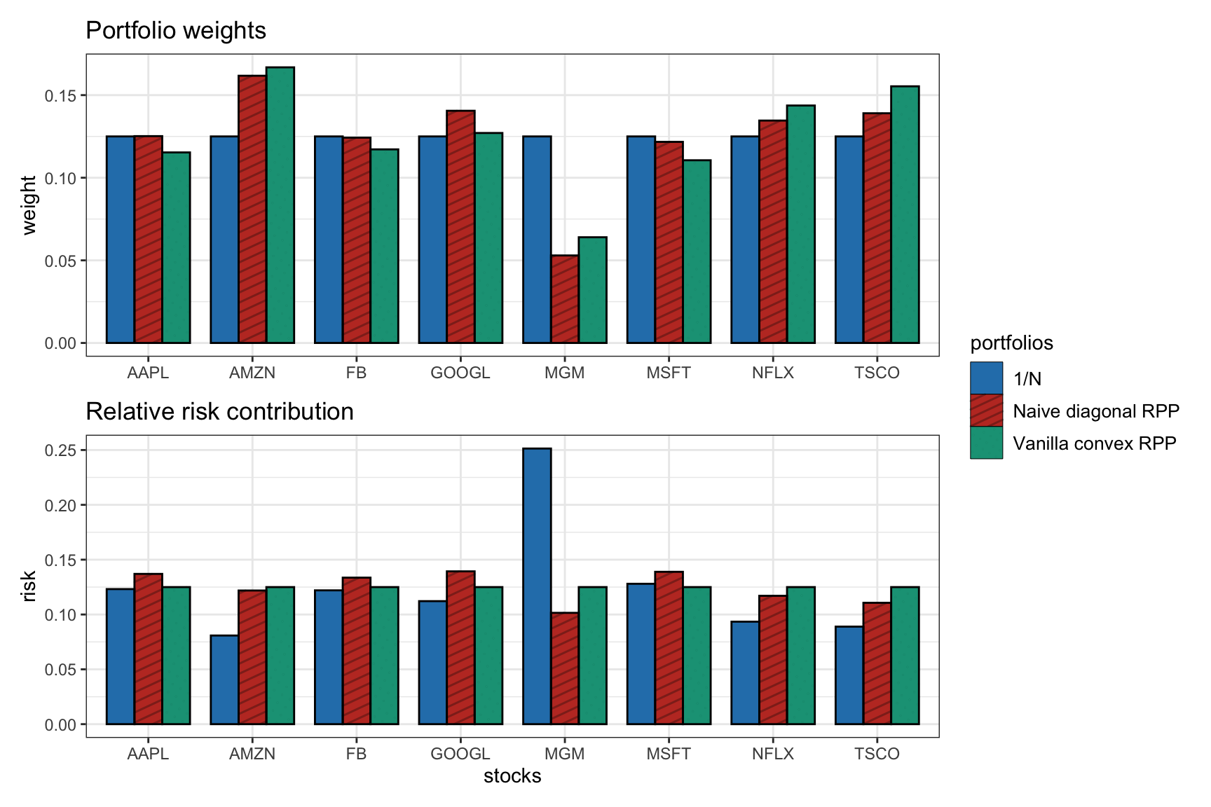
Figure 11.3: Portfolio allocation and risk contribution of the vanilla convex RPP compared to benchmarks (\(1/N\) portfolio and naive diagonal RPP).
11.6.3 Algorithms
As an alternative to using a general-purpose solver, we will now develop several practical iterative algorithms tailored to the problem formulations in (11.5) and (11.6) that produce a sequence of iterates \(\bm{x}^0, \bm{x}^1, \bm{x}^2,\dots\)
As the initial point of these iterative algorithms, we can use several options that attempt to approximately solve the system of nonlinear equations \(\bSigma\bm{x} = \bm{b}/\bm{x}\):
Naive diagonal solution: Inspired by the diagonal case \(\bSigma = \textm{Diag}(\bm{\sigma}^2)\), we can simply use \[ \bm{x}^0 = \sqrt{\bm{b}}/\bm{\sigma}. \]
Scaled heuristic for (11.5): For any given point \(\bar{\bm{x}}\), we can always find a more appropriate scaling factor \(t\) such that \(\bm{x}=t\bar{\bm{x}}\) satisfies the sum of the nonlinear equations \(\bm{1}^\T\bSigma\bm{x} = \bm{1}^\T(\bm{b}/\bm{x})\), leading to \(t = \sqrt{\bm{1}^\T(\bm{b}/\bar{\bm{x}})/\bm{1}^\T\bSigma\bar{\bm{x}}}\) and then \[ \bm{x}^0 = \bar{\bm{x}} \times \sqrt{\frac{\bm{1}^\T(\bm{b}/\bar{\bm{x}})}{\bm{1}^\T\bSigma\bar{\bm{x}}}}. \]
Scaled heuristic for (11.6): For any given point \(\bar{\bm{x}}\), we can always find a more appropriate scaling factor \(t\) such that \(\bm{x}=t\bar{\bm{x}}\) satisfies the sum of the nonlinear equations \(\bm{1}^\T\bSigma\bm{x} = \bm{1}^\T(\bm{b}/\bm{x}) \times \sqrt{\bm{x}^\T\bSigma\bm{x}}\), leading to \[ \bm{x}^0 = \bar{\bm{x}} \times \frac{\bm{1}^\T(\bm{b}/\bar{\bm{x}})}{\bm{1}^\T\bSigma\bar{\bm{x}}}\sqrt{\bar{\bm{x}}^\T\bSigma\bar{\bm{x}}}. \]
Diagonal row-sum heuristic: Using \(\textm{Diag}(\bSigma\bm{1})\) in lieu of \(\bSigma\) leads to \[ \bm{x}^0 = \sqrt{\bm{b}}/\sqrt{\bSigma\bm{1}}. \]
Newton’s Method
Newton’s method obtains the iterates based on the gradient \(\nabla f\) and the Hessian \({\sf H} f\) of the objective function \(f(\bm{x})\) as follows: \[\bm{x}^{k+1} = \bm{x}^{k} - \mathsf{H}f(\bm{x}^{k})^{-1} \nabla f(\bm{x}^{k}).\] For details on Newton’s method, the reader is referred to Section B.2 in Appendix B. The specific application of Newton’s method to risk parity portfolio was studied in detail in Spinu (2013).
In our case, the gradient and Hessian are easily computed as follows:
- For the function \(f(\bm{x}) = \frac{1}{2}\bm{x}^\T\bSigma\bm{x} - \bm{b}^\T\log(\bm{x})\) in (11.5): \[ \begin{aligned} \nabla f(\bm{x}) &= \bSigma\bm{x} - \bm{b}/\bm{x},\\ \mathsf{H}f(\bm{x}) &= \bSigma + \textm{Diag}(\bm{b}/\bm{x}^2). \end{aligned} \]
- For the function \(f(\bm{x}) = \sqrt{\bm{x}^\T\bSigma\bm{x}} - \bm{b}^\T\log(\bm{x})\) in (11.6): \[ \begin{aligned} \nabla f(\bm{x}) &= \bSigma\bm{x}/\sqrt{\bm{x}^\T\bSigma\bm{x}} - \bm{b}/\bm{x},\\ \mathsf{H}f(\bm{x}) &= \left(\bSigma - \bSigma\bm{x}\bm{x}^\T\bSigma/\bm{x}^\T\bSigma\bm{x}\right) / \sqrt{\bm{x}^\T\bSigma\bm{x}} + \textm{Diag}(\bm{b}/\bm{x}^2). \end{aligned} \]
Cyclical Coordinate Descent Algorithm
This method simply minimizes the function \(f(\bm{x})\) in a cyclical manner with respect to each element \(x_i\) of the variable \(\bm{x} = (x_1, \dots, x_N)\), while holding the other elements fixed. It is a particular case of the block coordinate descent (BCD) algorithm, also called the Gauss–Seidel method; for details, the reader is referred to Section B.6 in Appendix B.
This approach makes sense when the minimization with respect to a single element \(x_i\) becomes much easier. In particular, in our case the minimizer can be conveniently derived in closed form as follows (Griveau-Billion et al., 2013):
For the function \(f(\bm{x}) = \frac{1}{2}\bm{x}^\T\bSigma\bm{x} - \bm{b}^\T\log(\bm{x})\) in (11.5), the elementwise minimization becomes \[ \begin{array}{ll} \underset{x_i\ge0}{\textm{minimize}} & \frac{1}{2}x_i^2\bSigma_{ii} + x_i(\bm{x}_{-i}^\T\bSigma_{-i,i}) - b_i\log{x_i}, \end{array} \] where \(\bm{x}_{-i} = (x_1,\dots,x_{i-1}, x_{i+1},\dots,x_N)\) denotes the variable \(\bm{x}\) without the \(i\)th element and \(\bSigma_{-i,i}\) denotes the \(i\)th column of matrix \(\bSigma\) without the \(i\)th element. Setting the partial derivative with respect to \(x_i\) to zero gives us the second-order equation \[ \bSigma_{ii}x_i^2 + (\bm{x}_{-i}^\T\bSigma_{-i,i}) x_i - b_i = 0 \] with positive solution given by \[ x_i = \frac{-\bm{x}_{-i}^\T\bSigma_{-i,i}+\sqrt{(\bm{x}_{-i}^\T\bSigma_{-i,i})^2+ 4\bSigma_{ii} b_i}}{2\bSigma_{ii}}. \]
For the function \(f(\bm{x}) = \sqrt{\bm{x}^\T\bSigma\bm{x}} - \bm{b}^\T\log(\bm{x})\) in (11.6), the derivation follows similarly, with the update for \(x_i\) given by \[ x_i = \frac{-\bm{x}_{-i}^\T\bSigma_{-i,i}+\sqrt{(\bm{x}_{-i}^\T\bSigma_{-i,i})^2+ 4\bSigma_{ii} b_i\sqrt{\bm{x}^\T\bSigma\bm{x}}}}{2\bSigma_{ii}}. \]
The main issue with this method is that the elements of \(\bm{x}\) have to be updated sequentially at each iteration, which increases the computational complexity per iteration. One might be tempted to try a parallel update, but then convergence would not be guaranteed.
Parallel Update via MM
The reason why a parallel update cannot be implemented is that the term \(\bm{x}^\T\bSigma\bm{x}\) couples all the elements of \(\bm{x}\). One way to decouple these elements is via the majorization–minimization (MM) framework; for details on MM, the reader is referred to Section B.7 in Appendix B.
The MM method obtains the iterates \(\bm{x}^0, \bm{x}^1, \bm{x}^2,\dots\) by solving a sequence of simpler surrogate or majorized problems. In particular, the following majorizer is used for the term \(\bm{x}^\T\bSigma\bm{x}\) around the current point \(\bm{x} = \bm{x}^k\), that is, an upper-bound tangent at the current point: \[ \frac{1}{2}\bm{x}^\T\bSigma\bm{x} \leq \frac{1}{2}(\bm{x}^k)^\T\bSigma\bm{x}^k + (\bSigma\bm{x}^k)^\T(\bm{x} - \bm{x}^k) + \frac{\lambda_\textm{max}}{2}(\bm{x} - \bm{x}^k)^\T(\bm{x} - \bm{x}^k), \] where \(\lambda_\textm{max}\) is the largest eigenvalue of matrix \(\bSigma\). We can now solve our original problem by solving instead a sequence of majorized problems as follows:
The majorized problem corresponding to (11.5) is \[ \begin{array}{ll} \underset{\bm{x}\ge\bm{0}}{\textm{minimize}} & \frac{\lambda_\textm{max}}{2}\bm{x}^\T\bm{x} + \bm{x}^\T(\bSigma - \lambda_\textm{max}\bm{I})\bm{x}^k - \bm{b}^\T\log(\bm{x}), \end{array} \] from which setting the gradient to zero gives the second-order equation \[ \lambda_\textm{max}x_i^2 + ((\bSigma - \lambda_\textm{max}\bm{I})\bm{x}^k)_i x_i - b_i = 0 \] with positive solution \[ x_i = \frac{-((\bSigma - \lambda_\textm{max}\bm{I})\bm{x}^k)_i+\sqrt{((\bSigma - \lambda_\textm{max}\bm{I})\bm{x}^k)_i^2+ 4\lambda_\textm{max} b_i}}{2\lambda_\textm{max}}. \]
Similarly, forming the majorized problem for (11.6) and setting the gradient to zero gives the second-order equation \[ \lambda_\textm{max}x_i^2 + ((\bSigma - \lambda_\textm{max}\bm{I})\bm{x}^k)_i x_i - b_i \sqrt{(\bm{x}^k)^\T\bSigma\bm{x}^k} = 0 \] with positive solution \[ x_i = \frac{-((\bSigma - \lambda_\textm{max}\bm{I})\bm{x}^k)_i+\sqrt{((\bSigma - \lambda_\textm{max}\bm{I})\bm{x}^k)_i^2+ 4\lambda_\textm{max} b_i \sqrt{(\bm{x}^k)^\T\bSigma\bm{x}^k}}}{2\lambda_\textm{max}}. \]
Parallel Update via SCA
Another way to decouple the elements of \(\bm{x}\) in the term \(\bm{x}^\T\bSigma\bm{x}\) is via the successive convex approximation (SCA) framework; for details on SCA, the reader is referred to Section B.8 in Appendix B.
The SCA method obtains the iterates \(\bm{x}^0, \bm{x}^1, \bm{x}^2,\dots\) by solving a sequence of simpler surrogate problems. In particular, the following surrogate can be used for the term \(\bm{x}^\T\bSigma\bm{x}\) around the current point \(\bm{x} = \bm{x}^k\): \[ \frac{1}{2}\bm{x}^\T\bSigma\bm{x} \approx \frac{1}{2}(\bm{x}^k)^\T\bSigma\bm{x}^k + (\bSigma\bm{x}^k)^\T(\bm{x} - \bm{x}^k) + \frac{1}{2}(\bm{x} - \bm{x}^k)^\T\textm{Diag}(\bSigma)(\bm{x} - \bm{x}^k), \] where \(\textm{Diag}(\bSigma)\) is a diagonal matrix containing the diagonal of \(\bSigma\). We can now solve our original problems by solving instead a sequence of surrogate problems as follows:
The surrogate problem corresponding to (11.5) is \[ \begin{array}{ll} \underset{\bm{x}\ge\bm{0}}{\textm{minimize}} & \frac{1}{2}\bm{x}^\T\textm{Diag}(\bSigma)\bm{x} + \bm{x}^\T(\bSigma - \textm{Diag}(\bSigma))\bm{x}^k - \bm{b}^\T\log(\bm{x}), \end{array} \] from which setting the gradient to zero gives the second-order equation \[ \bSigma_{ii}x_i^2 + ((\bSigma - \textm{Diag}(\bSigma))\bm{x}^k)_i x_i - b_i = 0 \] with positive solution \[ x_i = \frac{-((\bSigma - \textm{Diag}(\bSigma))\bm{x}^k)_i+\sqrt{((\bSigma - \textm{Diag}(\bSigma))\bm{x}^k)_i^2+ 4\bSigma_{ii} b_i}}{2\bSigma_{ii}}. \]
Similarly, forming the surrogate problem for (11.6) and setting the gradient to zero gives the update \[ x_i = \frac{-((\bSigma - \textm{Diag}(\bSigma))\bm{x}^k)_i+\sqrt{((\bSigma - \textm{Diag}(\bSigma))\bm{x}^k)_i^2+ 4\bSigma_{ii} b_i \sqrt{(\bm{x}^k)^\T\bSigma\bm{x}^k}}}{2\bSigma_{ii}}. \]
11.6.4 Numerical Experiments
To evaluate the algorithms empirically, we use a universe of \(N=200\) stocks from the S&P 500 and compare their convergence in terms of iterations as well as CPU time (the latter is needed because each iteration may have a different computational cost depending on the method).
Effect of Initial Point
We start by evaluating in Figure 11.4 the effect of different initial points in Newton’s method for Spinu’s formulation (11.5). We can clearly observe that the effect is huge. Surprisingly, the naive diagonal solution, what would have seemed to be a good starting point, is the worst possible choice. The diagonal row-sum heuristic turns out to be an excellent choice and will be used hereafter.
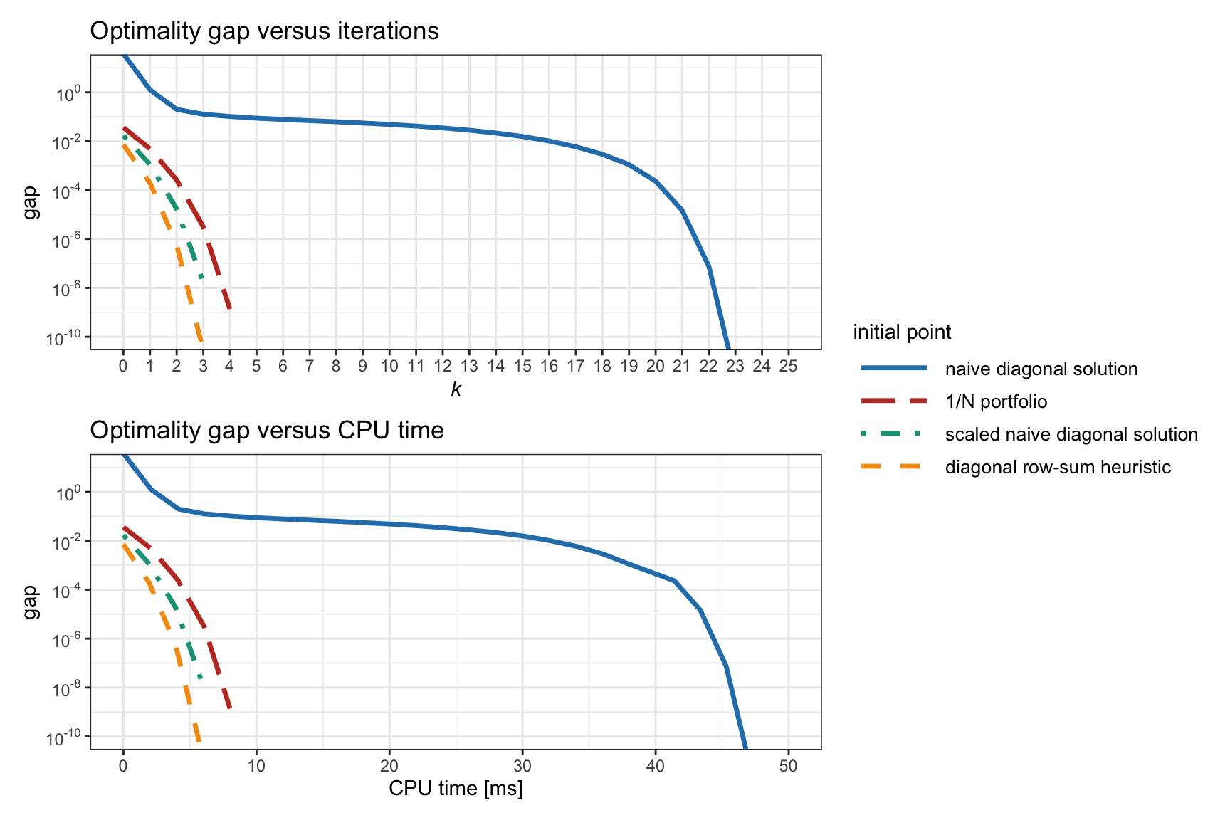
Figure 11.4: Effect of the initial point in Newton’s method for Spinu’s RPP formulation (11.5).
Comparison Between the Two Formulations (11.5) and (11.6)
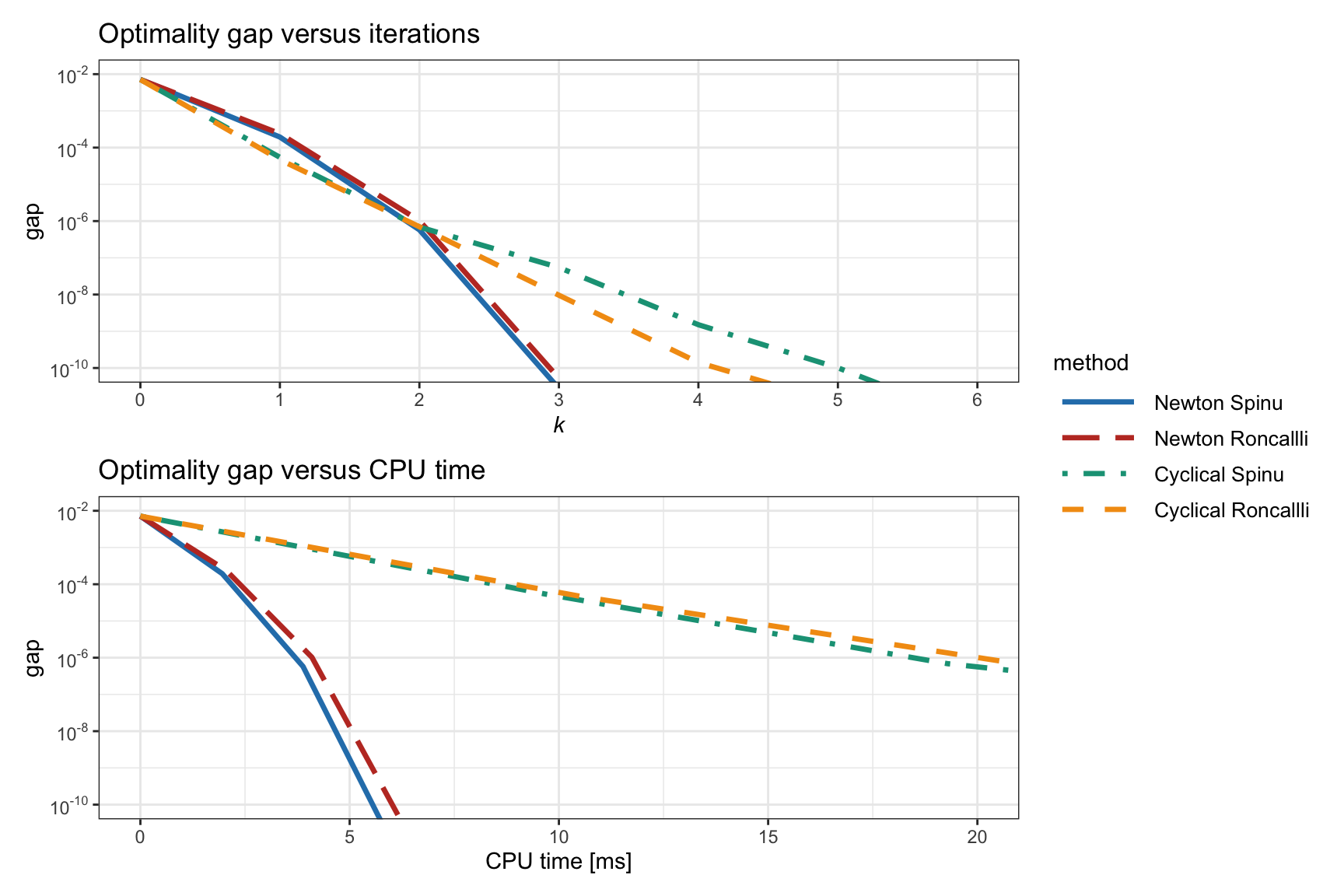
We continue by comparing in Figure 11.5 the difference between solving the two formulations in (11.5) (termed Spinu) and (11.6) (termed Roncalli) for Newton’s method and the cyclical coordinate descent method. We can observe that there is not much difference between the two formulations. Interestingly, the cyclical coordinate method shows the best convergence in terms of iterations, but the worst in terms of CPU time. However, a word of caution is needed here: in the cyclical update, each iteration requires updating each element sequentially and that requires a loop; it is well known that loops are slow in high-level programming languages like R or Python, but much faster in C++ or Rust. Thus, a more realistic comparison should be performed in a low-level programming language. As a first-order approximation, when implemented in a low-level programming language, one can expect the cyclical methods to perform very similarly to the parallel SCA methods.
Benefit of Reformulation in Terms of Correlation Matrix
Figure 11.6 explores the benefit of reformulating the problem in terms of the correlation matrix as in (11.4) instead of the covariance matrix – as already proposed in Spinu (2013) and numerically assessed in Choi and Chen (2022) – based on Newton’s method and MM for the formulation (11.5). A modest improvement is observed and will be used hereafter.
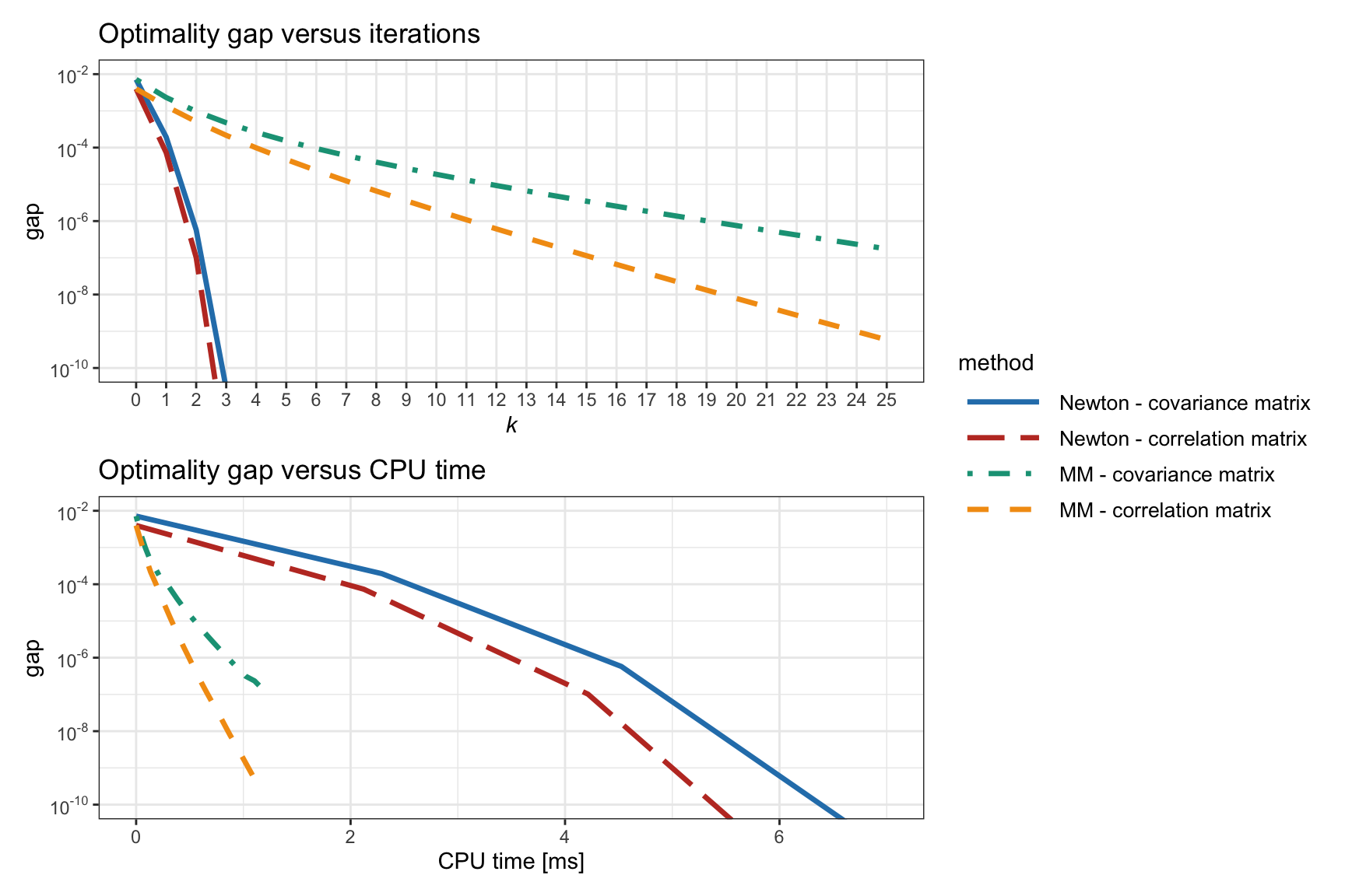
Figure 11.6: Effect of formulating the RPP problem in terms of the correlation matrix and the covariance matrix.
Benefit of the Normalization Step
The solution to \(\bSigma\bm{x} = \bm{b}/\bm{x}\) naturally satisfies \(\bm{x}^\T\bSigma\bm{x} = \bm{1}^\T\bm{b} = 1\). It was suggested in Choi and Chen (2022) to enforce such normalization after each iteration with the quadratic normalization step \[ \bm{x} \leftarrow \bm{x} \times \frac{1}{\sqrt{\bm{x}^\T\bSigma\bm{x}}}. \] This normalization has a complexity of \(\bigO(N^2)\), which is not insignificant. An alternative way is to enforce at each iteration \(\bm{1}^\T\bSigma\bm{x} = \bm{1}^\T(\bm{b}/\bm{x})\), leading to the linear normalization step \[ \bm{x} \leftarrow \bm{x} \times \sqrt{\frac{\bm{b}^\T(1/\bm{x})}{(\bm{1}^\T\bSigma)\bm{x}}}, \] which has a complexity of \(\bigO(N)\).
Figure 11.7 explores the benefit of introducing the normalization step (either quadratic or linear) for the formulation (11.5) based on the correlation matrix. A small improvement is observed in the case of the linear normalization.
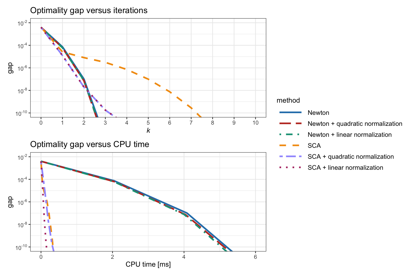
Figure 11.7: Effect of introducing a normalization step (quadratic or linear) in RPP algorithms.
Final Comparison of Selected Methods
Figure 11.8 shows the convergence of the Newton, MM, and SCA methods for problem (11.5), comparing the original version with the improved one (i.e., using the correlation matrix instead of the covariance matrix and using the linear normalization step). It seems that the best method is the improved SCA.
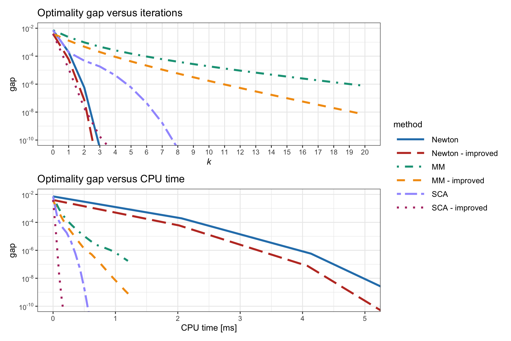
Figure 11.8: Convergence of different algorithms for the vanilla convex RPP.
Finally, it is insightful to study the convergence CPU time as a function of the problem dimension \(N\), as shown in Figure 11.9. Again, the improved SCA method seems the best, followed by the original SCA and the improved MM.
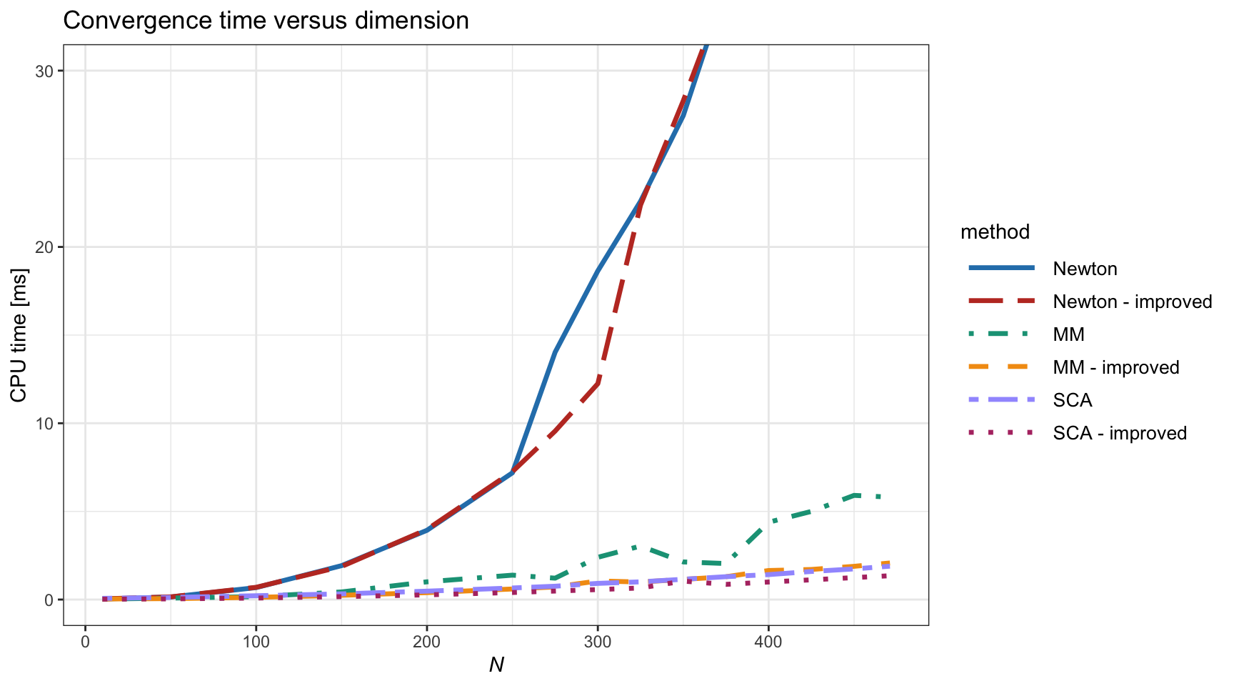
Figure 11.9: Computational cost vs. dimension \(N\) of different algorithms for the vanilla convex RPP.
References
In R, a general-purpose nonlinear multivariate root finder is provided by the function
multiroot()from the packagerootSolve. In MATLAB, we can use the functionfsolve().↩︎In R, there is a myriad of solvers, a typical example being the base function
optim(). In MATLAB, a similar function isfmincon().↩︎