\( \newcommand{\bm}[1]{\boldsymbol{#1}} \newcommand{\textm}[1]{\textsf{#1}} \def\T{{\mkern-2mu\raise-1mu\mathsf{T}}} \newcommand{\R}{\mathbb{R}} % real numbers \newcommand{\E}{{\rm I\kern-.2em E}} \newcommand{\w}{\bm{w}} % bold w \newcommand{\bmu}{\bm{\mu}} % bold mu \newcommand{\bSigma}{\bm{\Sigma}} % bold mu \newcommand{\bigO}{O} %\mathcal{O} \renewcommand{\d}[1]{\operatorname{d}\!{#1}} \)

2.2 Prices and returns

The price of an asset is arguably the most obvious quantity one can observe in financial markets. We denote it by \(p_{t}\), where \(t\) is the discrete time index (a continuous time index can also be used) corresponding to arbitrary periods such as minutes, hours, days, weeks, months, quarters, or years.

When it comes to modeling, it turns out that the logarithm of the prices, \[y_{t}\triangleq\textm{log}\; p_{t},\] is mathematically more convenient. In addition, using the logarithm has the advantage that a much wider dynamic range of the signal can be naturally represented (i.e., tiny values are amplified and large values are attenuated).

Some accessible textbooks that cover financial data modeling are (Cowpertwait and Metcalfe, 2009; Meucci, 2005; Ruppert and Matteson, 2015; Tsay, 2010), with more emphasis on the multi-asset case in (Lütkepohl, 2007; Tsay, 2013).

The simplest model for the log-prices is the random walk:

\[\begin{equation} y_{t} = \mu+y_{t-1} + \epsilon_{t}, \tag{2.1} \end{equation}\]

where \(\mu\) is the drift and \(\epsilon_{t}\) is the i.i.d. random noise. Figure 2.1 shows the daily prices of the stock index S&P 500⁴ over a span of more than a decade and Figure 2.2 shows the daily prices of Bitcoin⁵ over six years, both on a logarithmic scale (which is equivalent to plotting the log-prices on a linear scale).

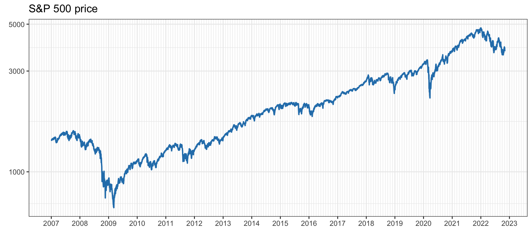
Figure 2.1: Price time series of S&P 500.

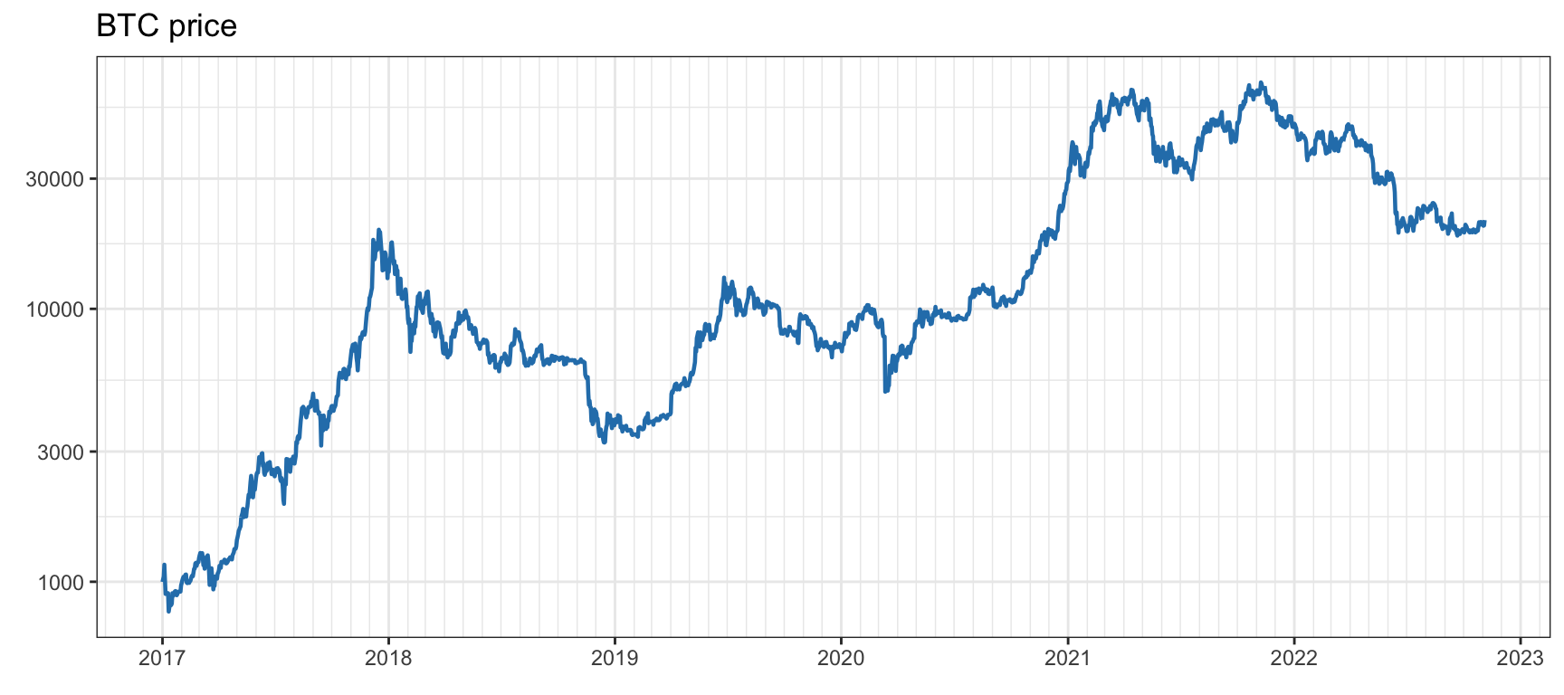
Figure 2.2: Price time series of Bitcoin.

Another key quantity is the price change, also called return, which, unlike the absolute price, exhibits some degree of stationarity and may be more convenient for mathematical modeling. Among the different definitions of returns (Ruppert and Matteson, 2015; Tsay, 2010), we will focus on two types that have important addivitive properties along two different domains:

• The linear return (a.k.a. simple or net return) is defined as \[r^{\textm{lin}}_t \triangleq\frac{p_{t}-p_{t-1}}{p_{t-1}}=\frac{p_{t}}{p_{t-1}}-1\] and has the property that it is additive among the assets (i.e., the overall linear return when investing in several assets equals the sum of the returns of the assets weighted according to the percentage of the budget invested in each). Thus, linear returns are key when dealing with the return of a portfolio of several assets (refer to Chapter 6 for details).

• The log-return (a.k.a. continuously compounded return) is defined as \[r^{\textm{log}}_t \triangleq y_{t}-y_{t-1}=\log\left(\frac{p_{t}}{p_{t-1}}\right)\] and has the property that is is additive along the time domain (i.e., the log-return of a long period equals the sum of the log-returns of the basic periods within the long period). Thus, log-returns are preferred when it comes to mathematical modeling of time series (refer to Chapters 3-4). For example, according to the previous random walk model in (2.1), the log-return is stationary: \[r^{\textm{log}}_t=y_{t}-y_{t-1}=\mu+\epsilon_{t}.\]

Interestingly, the simple return and log-return are related as \[r^{\textm{log}}_t = \log\left(1+r^{\textm{lin}}_t\right),\] which leads to the convenient approximation \(r^{\textm{log}}_t\approx r^{\textm{lin}}_t\), when \(r^{\textm{lin}}_t\) is small, as illustrated in Figure 2.3. The approximation is almost perfect when the magnitude of the return is less than 0.05 or 5%, then it slowly degrades.

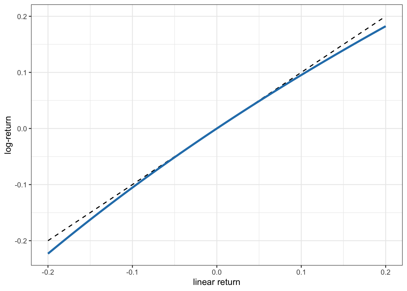
Figure 2.3: Approximation of log-return versus linear return.

Figure 2.4 shows the daily log-returns of the S&P 500 stock index over a span of more than a decade. One can easily observe the high-volatility period during global financial crisis in 2008, as well as the high peak in volatility in early 2020 due to the COVID-19 pandemic. Figure 2.2 shows the daily log-returns of Bitcoin over six years. Observe the Bitcoin flash crash on March 12, 2020, with a drop close to 50% in a single day.⁶

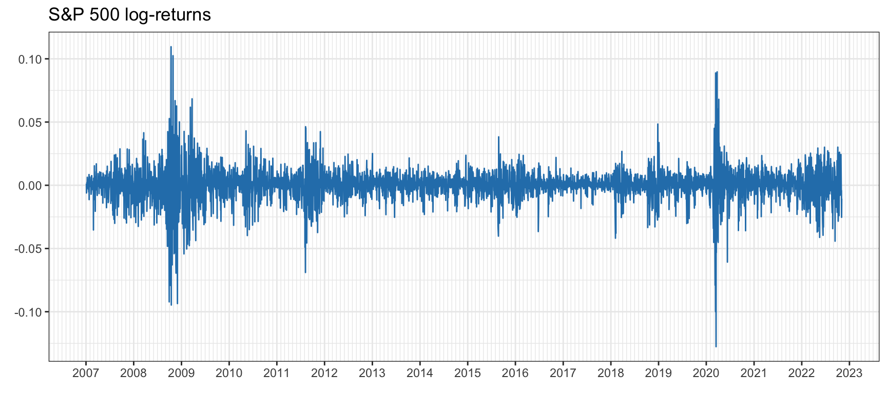
Figure 2.4: Daily log-return time series of S&P 500.

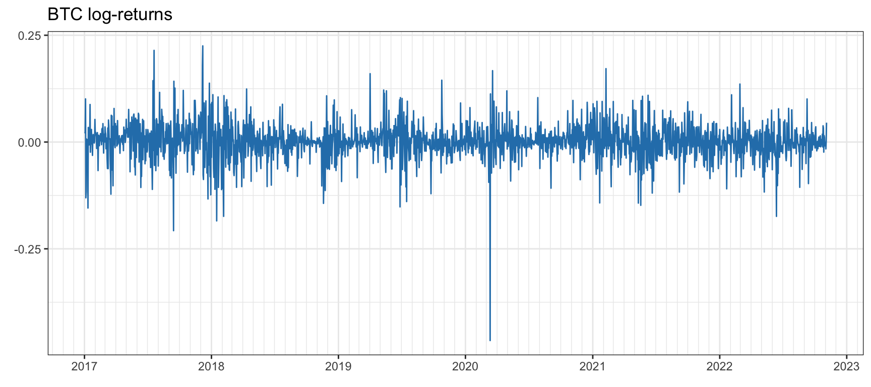
Figure 2.5: Daily log-return time series of Bitcoin.

It is insightful to compare the volatility levels for the two classes of assets. The annualized volatility of the S&P 500 stock index is on the order of 21%, whereas for Bitcoin it is around 78%. Generally speaking, a value of anywhere between 12% and 20% is considered low, whereas above 30% it is considered extremely volatile. Thus, the S&P 500 has a low volatility whereas Bitcoin is extremely volatile.

References

Cowpertwait, P. S. P., and Metcalfe, A. V. (2009). Introductory time series with R. Springer.

Lütkepohl, H. (2007). New introduction to multiple time series analysis. Springer.

Meucci, A. (2005). Risk and asset allocation. Springer.

Ruppert, D., and Matteson, S. D. (2015). Statistics and data analysis for financial engineering: With R examples. Springer.

Tsay, R. S. (2010). Analysis of financial time series. John Wiley & Sons.

Tsay, R. S. (2013). Multivariate time series analysis: With R and financial applications. John Wiley & Sons.

---

4. The Standard and Poor’s 500, or simply the S&P 500, is a stock market index of 500 of the largest companies listed on stock exchanges in the United States. It is one of the most commonly followed equity indices.↩︎

5. Bitcoin (BTC) is the first and most popular cryptocurrency. It was invented in 2008 by an unknown person or group of people using the name Satoshi Nakamoto. The currency began its use in 2009.↩︎

6. The flash crash of March 12, 2020, was triggered by COVID-19, since, just one day earlier, the World Health Organization (WHO) had announced that “COVID-19 can be characterized as a pandemic.”↩︎