12.3 Hierarchical clustering-based portfolios

$ \newcommand{\bm}[1]{\boldsymbol{#1}} \newcommand{\textm}[1]{\textsf{#1}} \def\T{{\mkern-2mu\raise-1mu\mathsf{T}}} \newcommand{\R}{\mathbb{R}} % real numbers \newcommand{\E}{{\rm I\kern-.2em E}} \newcommand{\w}{\bm{w}} % bold w \newcommand{\bmu}{\bm{\mu}} % bold mu \newcommand{\bSigma}{\bm{\Sigma}} % bold mu \newcommand{\bigO}{O} %\mathcal{O} \renewcommand{\d}[1]{\operatorname{d}\!{#1}} $

12.3 Hierarchical clustering-based portfolios

An alternative to using the noisy estimates of the mean vector $\bmu$ and covariance matrix $\bSigma$ in the mean–variance formulation is to design portfolios based on the graph of assets. This may produce more robust portfolios, more diversified, and with better risk-adjusted performance. Indeed, once the assets are hierarchically clustered, a variety of portfolios can be conveniently designed without relying so much on the noisy estimates of the mean vector and covariance matrix.

Hierarchical clustering aims at achieving diversification by a mechanism that distributes capital weights appropriately across the hierarchically nested clusters. The diversification scheme indicates which stocks are very isolated far away from the bulk of stocks and should receive a higher weight as they are contributors to diversification. The whole process can be visualized based on the hierarchical tree layout.

The general description of the hierarchical clustering-based portfolios is simple. The idea is to start with the total capital at the top and then proceed to allocate the capital through the hierarchical clustering along the dendrogram in a top-down manner. The starting point is the top giant cluster, which contains all the items, and the method proceeds down sequentially, where each cluster is successively divided into two sub-clusters. Every time a cluster is divided into two sub-clusters, the weight of the cluster has to be split into the two sub-clusters and the portfolios for the sub-clusters have to be designed.

The different hierarchical clustering-based portfolios (considered next in detail) are fully described by the following characteristics:

distance matrix: used to define the graph (e.g., correlation-based distance matrix in (12.1), distance matrix of the columns of such distance matrix as in (12.2), or obtained from some more sophisticated graph learning procedure);
linkage method: employed in the hierarchical clustering process (e.g., single, complete, average, or Ward);
clustering stopping criterion: used to stop the hierarchical clustering process (e.g., all the way down to single-item clusters or early stopping based on the gap statistic);
splitting criterion: to recursively split the assets (e.g., simply bisection or based on the dendrogram);
intra-weight allocation: used within clusters; and
inter-weight allocation: used across clusters.

The following subsections explore in detail several cases of hierarchical clustering-based portfolios, namely, the hierarchical $1/N$ portfolio, the hierarchical risk parity portfolio, and the hierarchical equal risk contribution portfolio.

12.3.1 Hierarchical $1/N$ portfolio

In 2011, a simple graph-based portfolio termed cluster-based waterfall portfolio was proposed in the PhD thesis (Papenbrock, 2011). The approach is based on the hierarchical tree obtained from the correlation-based distance matrix in (12.1). The allocation process goes over the dendrogram in a top-down manner, splitting the weights equally at each splitting point (i.e., the $1/N$ portfolio or equally-weighted portfolio from Section 6.4.3). Figure 12.4 illustrates this top-down process of equal weight splitting.

$Illustration of the hierarchical $1/N$ portfolio construction in a top-down manner.$

Figure 12.4: Illustration of the hierarchical $1/N$ portfolio construction in a top-down manner.

It is important to realize that the choice of linkage method has a significant effect on the concentration of the weight allocation as illustrated in Figure 12.5. Basically, the single linkage suffers from the “chaining” effect by which assets are branched out one by one, resulting in very high weights on some stocks; the complete linkage produces more even groups and weights; the average linkage lies somewhere in between, and Ward’s method is similar to the complete linkage producing slightly even more balanced groups and more equal weights. Note that the regular $1/N$ portfolio lies on the extreme of totally equalized weights, which amounts to not using any graph information at all, hence referred to as naive $1/N$ portfolio, as opposed to the hierarchical $1/N$ portfolio, which is based on the graph information.

$Chaining effect of different linkage methods on the hierarchical $1/N$ allocation.$

Figure 12.5: Chaining effect of different linkage methods on the hierarchical $1/N$ allocation.

Summary of the hierarchical $1/N$ portfolio (Papenbrock, 2011):

distance matrix: correlation-based distance matrix $D_{ij} = \sqrt{\frac{1}{2}(1 - \rho_{ij})}$ as in (12.1);
linkage method: recommended methods are the single linkage (for high risk investors willing to take high stakes in single assets) and Ward’s method (for risk averse investors with less concentration on single assets);
clustering stopping criterion: all the way down to single-item clusters;
splitting criterion: following the dendrogram;
intra-weight allocation: $1/N$ portfolio; and
inter-weight allocation: $1/N$ portfolio with $N=2$, i.e., 50% - 50% split at each branching.

Numerical results

We now compare different versions of the hierarchical $1/N$ portfolio along with some benchmarks. We first compare the hierarchical $1/N$ portfolio with the four different types of linkage methods along with the naive $1/N$ portfolio (illustrated in Figure 12.5). Figure 12.6 shows the portfolio weights: in this particular case the average linkage coincides with Ward’s method. Figure 12.7 shows the cumulative P&L and drawdown of the portfolios for a single illustrative backtest: as already indicated in the original publication (Papenbrock, 2011), Ward’s method is a good choice and will be used subsequently.

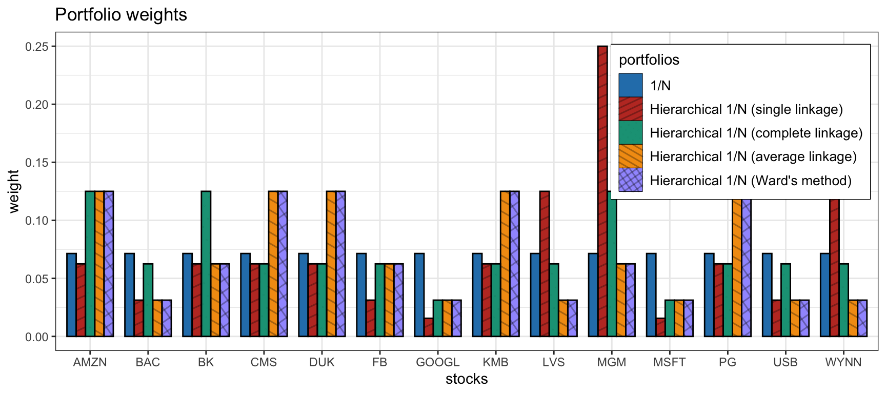
Figure 12.6: Portfolio allocation of hierarchical $1/N$ portfolios with different linkage methods.

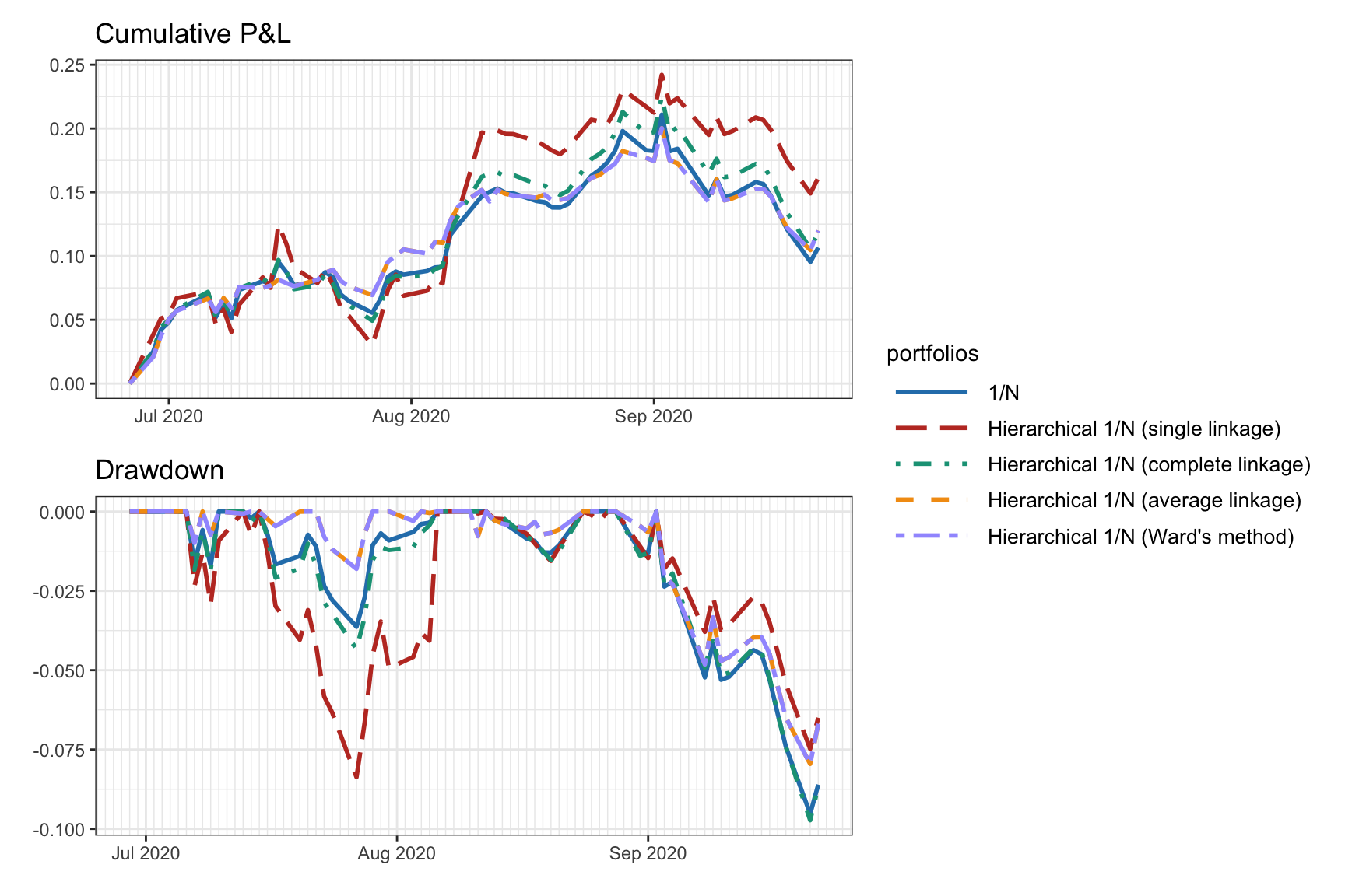
Figure 12.7: Backtest performance of hierarchical $1/N$ portfolios with different linkage methods.

Now we compare the use of the correlation-based distance matrix in (12.1), which was the choice in (Papenbrock, 2011), with the correlation-based distance-of-distance matrix in (12.2), as used in (López de Prado, 2016), as well as the graphs estimated via (12.3) and (12.4). Figure 12.8 compares the portfolio allocations, whereas Figure 12.9 shows the cumulative P&L and drawdown of the portfolios for a single illustrative backtest. In this particular case, it seems that the simple correlation-based distance-of-distance matrix in (12.2) shows a better drawdown, but more exhaustive backtests are necessary before concluding anything.

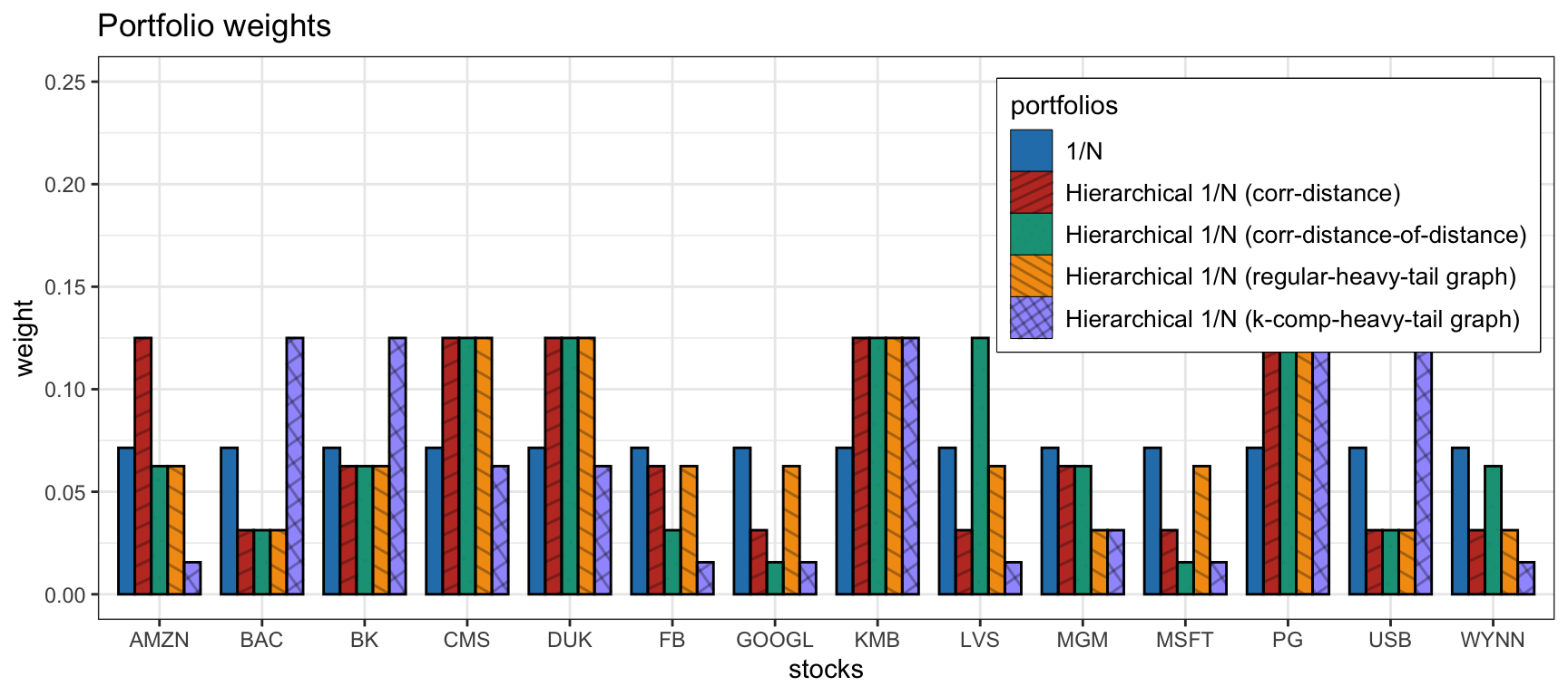
Figure 12.8: Portfolio allocation of hierarchical $1/N$ portfolios with different distance matrices.

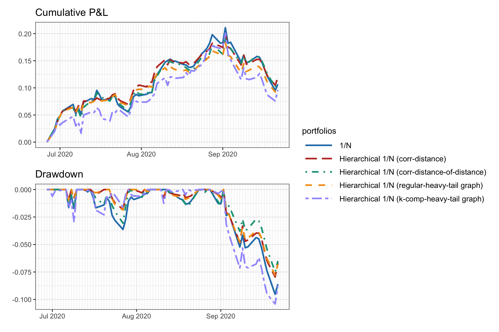
Figure 12.9: Backtest performance of hierarchical $1/N$ portfolios with different distance matrices.

Finally, we compare the selected version of the hierarchical $1/N$ portfolio (using Ward’s method for the linkage and the correlation-based distance-of-distance matrix in (12.2)) with the following benchmarks: naive $1/N$ portfolio, global minimum variance portfolio (GMVP), and Markowitz mean–variance portfolio (MVP). Figure 12.10 compares the portfolio allocations, from where we can clearly see the difference in diversification. Figure 12.11 shows the cumulative P&L and drawdown of the portfolios for a single illustrative backtest: as expected, the MVP shows the worst drawdown (due to the sensitivity to the estimation of $\bmu$), followed by GMVP and $1/N$ portfolio, with the hierarchical $1/N$ portfolio having the mildest drawdown. Nevertheless, the reader is reminded that this is just a single anecdotal backtest and a proper empirical evaluation based on multiple randomized backtests is necessary as explored further later in Section 12.4.

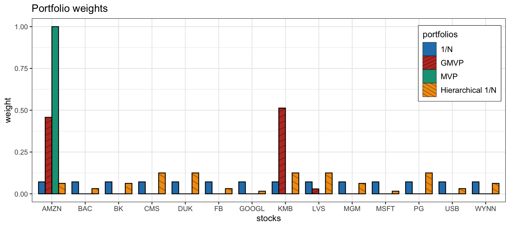
Figure 12.10: Portfolio allocation of hierarchical $1/N$ portfolio along benchmarks.

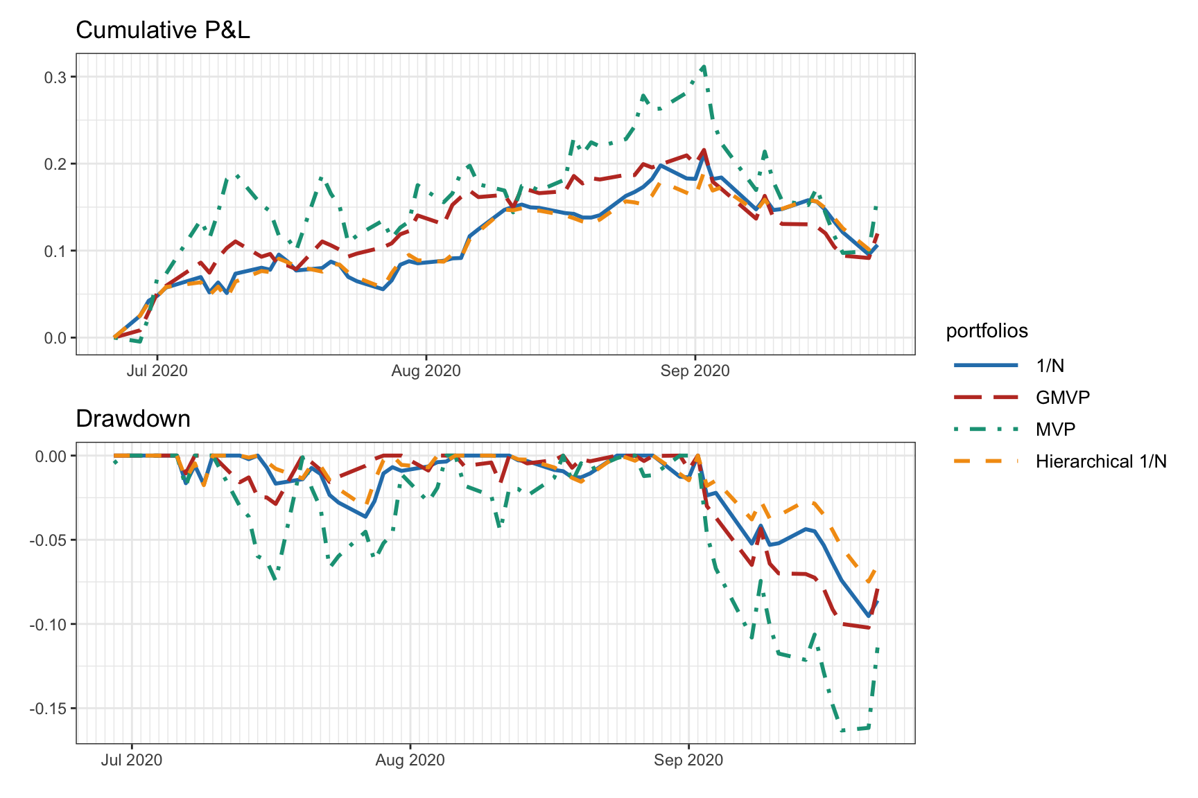
Figure 12.11: Backtest performance of hierarchical $1/N$ portfolio along benchmarks.

12.3.2 Hierarchical risk parity (HRP) portfolio

In 2016, a graph-based portfolio was proposed in (López de Prado, 2016) called hierarchical risk parity (HRP) portfolio. The method is based on the hierarchical tree obtained from the correlation-based distance-of-distance matrix in (12.2) and the single linkage method. The allocation process goes over the dendrogram from a top-down manner, splitting the weights based on the inverse-variance portfolio (IVarP).

Before going into the details of HRP, let us start by recalling that the global minimum variance portfolio with budget constraint is formulated (see Section 6.5.1 in Chapter 6) as \[ \begin{array}{ll} \underset{\w}{\textm{minimize}} & \w^\T\bSigma\w\\ \textm{subject to} & \w^\T\bm{1} = 1, \end{array} \] with solution \[ \w = \frac{\bSigma^{-1}\bm{1}}{\bm{1}^\T\bSigma^{-1}\bm{1}}. \] If the covariance matrix $\bSigma$ is diagonal, with diagonal elements denoted by $\bm{\sigma}^2 = \textm{diag}(\bSigma)$, then the solution simplifies to the inverse-variance portfolio: \[\begin{equation} \w = \frac{\bm{\sigma}^{-2}}{\bm{1}^\T\bm{\sigma}^{-2}}, \tag{12.5} \end{equation}\] which, for the particular case of $N=2$ assets, becomes \[\begin{equation} \begin{bmatrix} w_1\\ w_2 \end{bmatrix} = \begin{bmatrix} \sigma_1^{-2}/(\sigma_1^{-2} + \sigma_2^{-2})\\ \sigma_2^{-2}/(\sigma_1^{-2} + \sigma_2^{-2}) \end{bmatrix} = \begin{bmatrix} \sigma_2^{2}/(\sigma_1^{2} + \sigma_2^{2})\\ \sigma_1^{2}/(\sigma_1^{2} + \sigma_2^{2}) \end{bmatrix}. \tag{12.6} \end{equation}\]

We are now ready to go over the HRP portfolio design process. Similarly to the hierarchical $1/N$ portfolio, the allocation process goes over the dendrogram in a top-down manner, splitting the weights at each splitting point. A first difference in the HRP method proposed in (López de Prado, 2016) is that the splitting is based on bisection (i.e., dividing the items into two halves) rather than the natural structure given by the dendrogram, as illustrated in Figure 12.12. In the bisection splitting, the dendrogram still contributes with the ordering of the assets. A priori, one cannot say which of the two methods will perform better and this will be later empirically evaluated. The second main difference is that instead of basing the weight splitting on the $1/N$ portfolio with $N=2$, which leads to a 50% - 50% splitting of the budget, the weight splitting is based on the IVarP with $N=2$ in (12.6). In order to compute the variances of the two branches $\sigma_1^{2}$ and $\sigma_2^{2}$, the method uses at each branch the IVarP (12.5) (which presumably is not too far from the optimal GMVP since we are dealing with a quasi-diagonal matrix). Algorithm 12.1 formalizes the HRP portfolio construction.

Figure 12.12: Comparison of bisection splitting and dendrogram-based splitting.

Summary of the HRP portfolio (López de Prado, 2016):

distance matrix: correlation-based distance-of-distance matrix in (12.2);
linkage method: single linkage;
clustering stopping criterion: all the way down to single-item clusters;
splitting criterion: directly bisection ignoring the grouping sizes from the dendrogram;
intra-weight allocation: IVarP; and
inter-weight allocation: IVarP for $N=2$ as in (12.6).

The HRP portfolio can be interpreted as a refined version of the inverse-variance portfolio. Indeed, at each step, given two subsets, the portfolio weights are scaled based on the inverse of the variances while ignoring the correlation between the subsets (presumably these subsets are not highly correlated). The only point where correlations are considered is in the computation of the variances of each of the subsets. In fact, when the covariance matrix is diagonal, then the inverse-variance portfolio, the global minimum variance portfolio, and the HRP portfolio coincide. A connection between the HRP portfolio and the minimum-variance portfolio is further outlined in Section 12.3.4.

Algorithm 12.1: HRP portfolio.

Initialize list of groups of items $\mathcal{L} = \{L_0\}$, with $L_0 = \{1,\dots,N\}$, and unit weights $\w = \bm{1}$;

repeat for each tuple $L_i \in \mathcal{L}$ with $|L_i| > 1$:

Partition $L_i$ into two subsets, $L_i^{(1)}$ and $L_i^{(2)}$; two options are:
- bisection split: following the dendrogram ordering, simply split it into two subsets of approximately equal size: $|L_i^{(1)}| = \textm{round}(|L_i|/2)$;
- dendrogram split: follow the dendrogram split of this set into two subsets (i.e., not only ordering but size of subsets too);
Define the variance of each subset $L_i^{(j)}, j=1,2$, as ${\tilde{\sigma}_i^2}^{(j)} = \tilde{\w}_i^{(j)\T}\bSigma_i^{(j)}\tilde{\w}_i^{(j)}$, where $\bSigma_i^{(j)}$ is the covariance matrix of the elements in $L_i^{(j)}$ and $\tilde{\w}_i^{(j)}$ is the inverse-variance portfolio in (12.5);
Compute the split factor as in (12.6): $\alpha_i = {\tilde{\sigma}_i^2}^{(2)}/({\tilde{\sigma}_i^2}^{(1)} + {\tilde{\sigma}_i^2}^{(2)})$;
Re-scale elements $n \in L_i^{(1)}$ in $\w$ by a factor of $\alpha_i$ and elements $n \in L_i^{(2)}$ in $\w$ by a factor of $(1- \alpha_i)$;

until $|L_i| = 1, \forall L_i \in L$;

Numerical results

We now compare the HRP portfolios (both with bisection split and dendrogram split) with the following benchmarks: global minimum variance portfolio (GMVP) and inverse-variance portfolio (IVarP).

Figure 12.13 shows the portfolio weights. The GMVP concentrates most of the weights into two assets, whereas the rest are more diversified. The HRP portfolios do not differ too much from the IVarP. Figure 12.14 shows the cumulative P&L and drawdown of the portfolios for a single illustrative backtest. The HRP portfolios seem to slightly improve on the IVarP; in addition, the graphs estimated via (12.3) and (12.4) seem to be better than the correlation-based distance-of-distance matrix in (12.2).

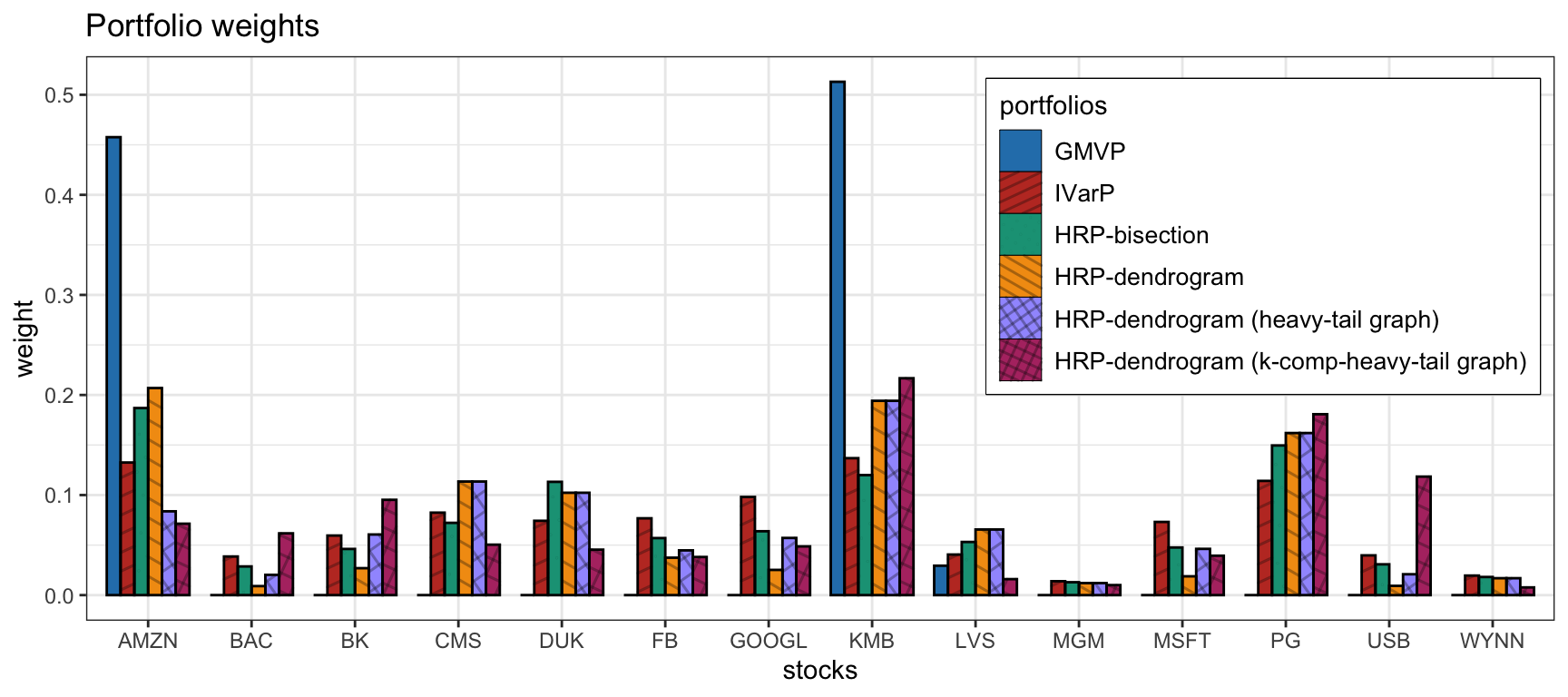
Figure 12.13: Portfolio allocation of HRP portfolios and benchmarks.

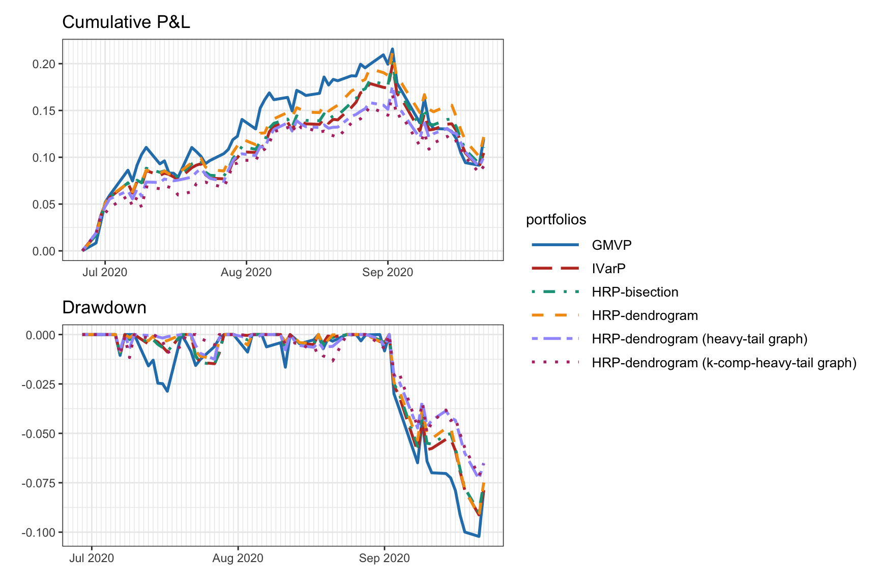
Figure 12.14: Backtest performance of HRP portfolios and benchmarks.

12.3.3 Hierarchical equal risk contribution (HERC) portfolio

In 2018, a refined and extended version of the hierarchical $1/N$ portfolio of Section 12.3.1 and the HRP portfolio of Section 12.3.2 was proposed in (Raffinot, 2018b) called hierarchical equal risk contribution (HERC) portfolio. Basically, the main two differences are:

Early stopping in the hierarchical clustering to automatically select the appropriate number of clusters based on the gap statistic (Tibshirani et al., 2001), technique already used in the hierarchical clustering asset allocation (HCAA) (Raffinot, 2018a), as opposed to clustering all the way down to single assets as typically done in hierarchical clustering.
Use of a general equal risk contribution to split the weights at each splitting point (which can be based on alternative measures of risk to the variance used in (12.6), such as standard deviation, conditional value-at-risk, conditional drawdown-at-risk, etc.: \[\begin{equation} \begin{bmatrix} w_1\\ w_2 \end{bmatrix} = \begin{bmatrix} \textm{RC}_1/(\textm{RC}_1 + \textm{RC}_2)\\ \textm{RC}_2/(\textm{RC}_1 + \textm{RC}_2) \end{bmatrix}, \tag{12.7} \end{equation}\] where $\textm{RC}_i$ denotes the risk contribution of of the $i$th cluster. Observe that if $\textm{RC}_i = 1/\sigma_i^{2}$, then we recover (12.6).

The main findings in (Raffinot, 2018b) can be summarized as follows:

“the hierarchical $1/N$ portfolio is difficult to beat, but HERC portfolios based on downside risk measures achieve statistically better risk-adjusted performances, especially those based on the conditional drawdown-at-risk.”

Figure 12.15 illustrates the effect of early stopping in the hierarchical clustering process with a hierarchical $1/N$ portfolio. In particular a toy dendrogram is considered with five assets grouped into three and two clusters.

Figure 12.15: Effect of early stopping in the hierarchical clustering process.

Summary of the HERC portfolio (Raffinot, 2018b):

distance matrix: correlation-based distance-of-distance matrix in (12.2);
linkage method: Ward’s method;
clustering stopping criterion: gap statistic (Tibshirani et al., 2001);
splitting criterion: following the dendrogram;
intra-weight allocation: $1/N$ portfolio; and
inter-weight allocation: equal risk constribution as in (12.7).

Numerical results

For simplicity, for the weight splitting we simply use the two risk contribution measures: $\textm{RC}_i = 1$ and $\textm{RC}_i = 1/\sigma_i^{2}$, leading to the 50% - 50% split as in the hierarchical $1/N$ portfolio and to (12.6) as in the HRP portfolio.

We now compare the HERC portfolios (both with bisection split and dendrogram split) with the following benchmarks: $1/N$ portfolio, hierarchical $1/N$ portfolio, inverse-variance portfolio (IVarP), and HRP portfolio. Figure 12.16 shows the portfolio weights, whereas Figure 12.17 shows the cumulative P&L and drawdown of the portfolios for a single illustrative backtest. It is difficult to conclude anything from this single backtest and more exhaustive backtests are necessary.

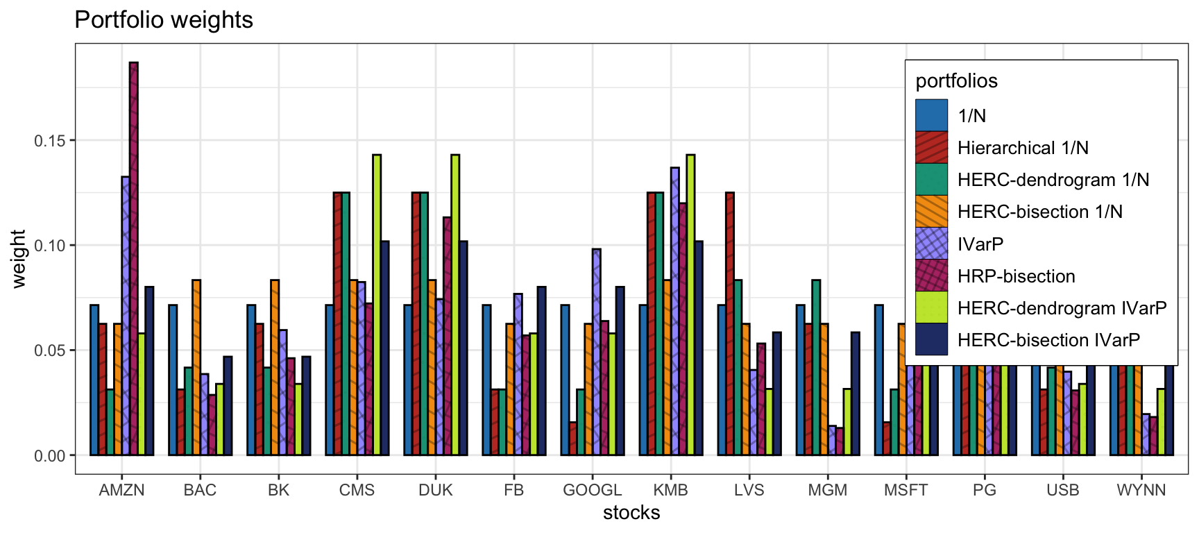
Figure 12.16: Portfolio allocation of HERC portfolios and benchmarks.

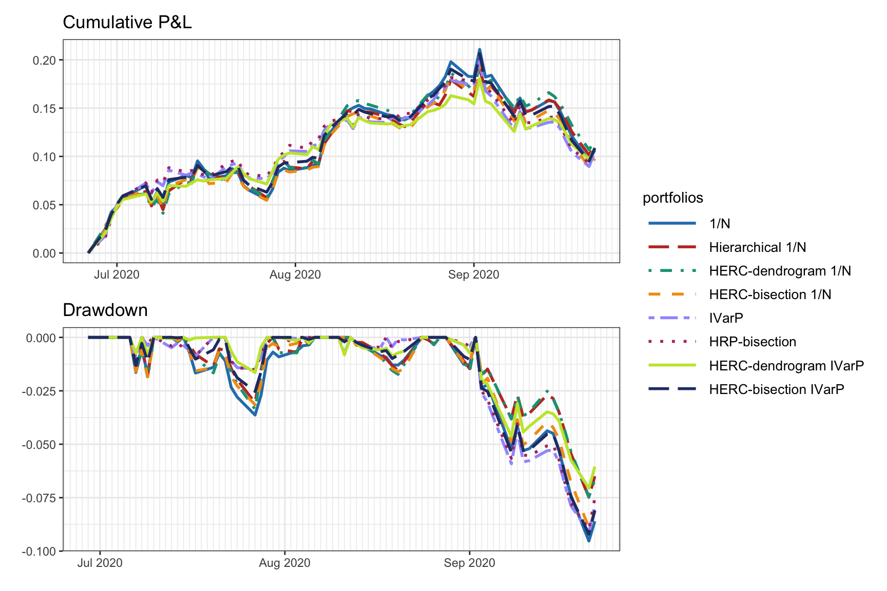
Figure 12.17: Backtest performance of HERC portfolios and benchmarks.

12.3.4 From portfolio risk minimization to hierarchical portfolios

The essence of the hierarchical portfolios covered in this section lies on successive partitioning of the set of assets with a proper inter-set capital allocation and intra-set portfolio allocation. To be more specific, at each round of this successive partitioning, we partition a set of assets, with covariance matrix $\bSigma$, into two subsets $A$ and $B$, with covariance matrices $\bSigma_A$ and $\bSigma_B$, respectively. Then, the portfolio is constructed as \[\begin{equation} \w \propto \begin{bmatrix} \frac{1}{\nu(\bSigma_A)} \w(\bSigma_A)\\[0.2em] \frac{1}{\nu(\bSigma_B)} \w(\bSigma_B) \end{bmatrix}, \tag{12.8} \end{equation}\] where $\nu\left(\cdot\right)$ and $\w\left(\cdot\right)$ denote some measure of risk and portfolio construction, respectively, for a set of assets with given covariance matrix. The first component $1/\nu(\cdot)$ provides the capital allocation into the two subsets (inversely proportional to the risk), whereas the second component $\w(\cdot)$ gives the (normalized) portfolio allocation for each subset.

The particular form of $\nu(\cdot)$ and $\w(\cdot)$ in (12.8) depends on each type of hierarchical portfolio. For example, in the case of the HRP portfolio covered in Section 12.3.2:

the intra-weight (normalized) allocation is given by the inverse-variance portfolio (12.5), \[ \w(\bSigma) = \frac{\bm{\sigma}^{-2}}{\bm{1}^\T \bm{\sigma}^{-2}}, \] where $\bm{\sigma}^2 = \textm{diag}(\bSigma)$ denotes the variance of the assets, and
the measure of risk (whose inverse gives the capital or inter-weight allocation) is measured by the variance (12.6), \[ \nu\left(\bSigma\right) = \w(\bSigma)^\T\,\bSigma\,\w(\bSigma). \]

However, the basic structure of hierarchical portfolios (12.8) is heuristic and suboptimal, which is understandable since the motivation was not optimality but stability against estimation errors. One reason for the lack of optimality can be seen in the fact that the portfolios in each of the two groups, $\w(\bSigma_A)$ and $\w(\bSigma_B)$, are oblivious to each other and the two groups are only jointly adjusted in the final normalization step of (12.8) (note the notation $\propto$ which requires a normalization that depends on all the elements). On the other hand, portfolios designed based on the minimization of some properly chosen measure of risk are not heuristic by definition but optimal according to the design criterion. Can we make an explicit connection between the two paradigms? Can we somehow derive an expression similar to (12.8) but more formally justified and optimally chosen?

A positive answer was provided in (Cotton, 2023) as described next. Consider the global minimum variance portfolio (see Section 6.5.1 in Chapter 6): \[ \begin{array}{ll} \underset{\w}{\textm{minimize}} & \w^\T\bSigma\w\\ \textm{subject to} & \w^\T\bm{1} = 1. \end{array} \] Interestingly, by partitioning $\bSigma$ as \[ \bSigma = \begin{bmatrix} \bSigma_A & \bSigma_{AB}\\ \bSigma_{BA} & \bSigma_{B} \end{bmatrix}, \] the optimal solution can be written (up to a scaling factor) in a form reminiscent to (12.8) as \[ \w \propto \bSigma^{-1}\bm{1} = \begin{bmatrix} (\bSigma_A^c)^{-1} \bm{b}_A\\ (\bSigma_B^c)^{-1} \bm{b}_B \end{bmatrix}, \] where $\bSigma_A^c$ and $\bSigma_B^c$ are the Schur complements of $\bSigma_A$ and $\bSigma_B$,⁵⁶ respectively, \[ \begin{aligned} \bSigma_A^c &= \bSigma_A - \bSigma_{AB}\bSigma_B^{-1}\bSigma_{BA}\\ \bSigma_B^c &= \bSigma_B - \bSigma_{BA}\bSigma_A^{-1}\bSigma_{AB}, \end{aligned} \] and \[ \begin{aligned} \bm{b}_A &= \bm{1} - \bSigma_{AB}\bSigma_B^{-1}\bm{1}\\ \bm{b}_B &= \bm{1} - \bSigma_{BA}\bSigma_A^{-1}\bm{1}. \end{aligned} \]

Finally, this optimal solution can be further rewritten in a form similar to (12.8) as \[\begin{equation} \w \propto \begin{bmatrix} \frac{1}{\nu(\bSigma_A^c, \bm{b}_A)} \w(\bSigma_A^c, \bm{b}_A)\\[0.5em] \frac{1}{\nu(\bSigma_B^c, \bm{b}_B)} \w(\bSigma_B^c, \bm{b}_B) \end{bmatrix}, \tag{12.9} \end{equation}\] where the (normalized) allocation is \[ \w(\bSigma, \bm{b}) = \frac{\bSigma^{-1}\bm{b}}{\bm{b}^\T\bSigma^{-1}\bm{b}} \] and the measure of risk is \[ \nu(\bSigma, \bm{b}) = \left(\w(\bSigma, \bm{b})\right)^\T\bSigma\,\w(\bSigma, \bm{b}) = \frac{1}{\bm{b}^\T\bSigma^{-1}\bm{b}}. \]

At this point it is important to realize that optimal portfolio in (12.9) becomes a hierarchical portfolio (12.8) if one replaces $\bSigma_A^c \rightarrow \bSigma_A$ and $\bm{b}_A \rightarrow \bm{1}$ (and similarly for $\bSigma_B^c$ and $\bm{b}_B$). This observation naturally leads to the idea of transitioning from one set of parameters to the other in a smooth way to provide a continuum ranging from a hierarchical portfolio to a minimum risk portfolio as some scalar parameter $\gamma$ goes from 0 to 1. There are multiple ways of doing such a smooth transition; some examples include:

convex combination: \[ \begin{aligned} \bSigma_A^{(\gamma)} &= (1 - \gamma) \bSigma_A + \gamma \bSigma_A^c = \bSigma_A - \gamma \bSigma_{AB}\bSigma_B^{-1}\bSigma_{BA}\\ \bm{b}_A^{(\gamma)} &= (1 - \gamma) \bm{1} + \gamma \bm{b}_A = \bm{1} - \gamma \bSigma_{AB}\bSigma_B^{-1}\bm{1}; \end{aligned} \]
geodesic-convex combination (Wiesel, 2012a): \[ \begin{aligned} \bSigma_A^{(\gamma)} &= \bSigma_A^{1/2} \left(\bSigma_A^{-1/2} \bSigma_A^c \bSigma_A^{-1/2}\right)^\gamma \bSigma_A^{1/2}\\ \bm{b}_A^{(\gamma)} &= \bm{b}_A^\gamma, \end{aligned} \] where the matrix power is defined via the power of the eigenvalues.

References

Cotton, P. (2023). A unification of machine learning and optimization-based portfolio construction.

López de Prado, M. (2016). Building diversified portfolios that outperform out of sample. Journal of Portfolio Management, 42(4), 59–69.

Papenbrock, J. (2011). Asset clusters and asset networks in financial risk management and portfolio optimization (PhD thesis). Karlsruher Institute für Technologie.

Raffinot, T. (2018a). Hierarchical clustering-based asset allocation. The Journal of Portfolio Management, 44(2), 89–99.

Raffinot, T. (2018b). The hierarchical equal risk contribution portfolio. SSRN Electronic Journal.

Tibshirani, R., Walther, G., and Hastie, T. (2001). Estimating the number of clusters in a data set via the gap statistic. Journal of the Royal Statistical Society. Series B: Statistical Methodology, 63(2), 411–423.

Wiesel, A. (2012a). Geodesic convexity and covariance estimation. IEEE Transactions on Signal Processing, 60(12), 6182–6189.

The Schur-complement of a block matrix is a key tool in the fields of numerical analysis, statistics, and matrix analysis. For our motivation, it suffices to know that it naturally appears in the inverse of a $2\times2$ matrix: \[ \begin{bmatrix} \bSigma_A & \bSigma_{AB}\\ \bSigma_{BA} & \bSigma_{B} \end{bmatrix}^{-1} = \begin{bmatrix} \left(\bSigma_A - \bSigma_{AB}\bSigma_B^{-1}\bSigma_{BA}\right)^{-1} & 0\\ 0 & \left(\bSigma_B - \bSigma_{BA}\bSigma_A^{-1}\bSigma_{AB}\right)^{-1} \end{bmatrix}\cdot \begin{bmatrix} \bm{I} & -\bSigma_{AB}\bSigma_B^{-1}\\ \bSigma_{BA}\bSigma_A^{-1} & \bm{I} \end{bmatrix}. \] ↩︎

Portfolio Optimization