14.3 Portfolio Resampling
We will first give an overview of resampling methods in statistics and then apply them to portfolio optimization.
14.3.1 Resampling Methods
Estimating a parameter \(\bm{\theta}\) with the value \(\hat{\bm{\theta}}\) is of little use if one does not know how good that estimate is. In statistical inference, confidence intervals are key as they allow us to localize the true parameter on some interval with, say, 95% confidence. Traditionally, the derivation and analysis of confidence intervals was very theoretical with heavy use of mathematics. Resampling methods, instead, resort to computer-based numerical techniques for assessing statistical accuracy without formulas (Efron and Tibshirani, 1993).
In statistics, resampling is the creation of new samples based on a single observed sample block. Suppose we have \(n\) observations, \(\bm{x}_1,\dots,\bm{x}_n\), of a random variable \(\bm{x}\) from which we estimate some parameters \(\bm{\theta}\) as \[ \hat{\bm{\theta}} = f(\bm{x}_1,\dots,\bm{x}_n), \] where \(f(\cdot)\) denotes the estimator. The estimation \(\hat{\bm{\theta}}\) is a random variable because it is based on \(n\) random variables. It may seem that the only possible way to characterize the distribution of the estimation would be to somehow have access to more realizations of the random variable \(\bm{x}\). However, this is precisely when resampling methods help to do some “magic.” The most popular methods include cross-validation and the bootstrap (Efron and Tibshirani, 1993).
Cross-Validation
Cross-validation is a type of resampling method widely used in portfolio backtesting (see Chapter 8) and machine learning (see Chapter 16). The idea is simple and consists of dividing the \(n\) observations into two groups: a training set for fitting or learning the estimator \(f(\cdot)\) and a validation set for assessing its performance. This process can be repeated multiple times to provide multiple realizations of the performance value, which can then be used to compute the empirical performance. For example, \(k\)-fold cross-validation divides the set into \(k\) subsets, where each is held back in turn as the validation set while using the others for training. Leave-one-out cross-validation is an extreme case where the original dataset of \(n\) observations is divided into \(k=n\) subsets, which means that for each subset a single observation is held back from the training process and used later for validation.
The Bootstrap
The bootstrap is a type of resampling method proposed in 1979 by Efron, which appears truly magical but it is nevertheless based on sound statistical theory (Efron, 1979). In fact, the name itself (bootstrap) figuratively refers to the seemingly impossible task of lifting oneself by pulling on one’s bootstraps.
The idea of the bootstrap is to mimic the original sampling process (from which the original \(n\) observations \(\bm{x}_1,\dots,\bm{x}_n\) were generated) by sampling these realizations \(n\) times with replacement (some samples will be selected multiple times while others will not be used). This procedure is repeated \(B\) times to obtain the bootstrap samples, \[ \big(\bm{x}_1,\dots,\bm{x}_n\big) \rightarrow \left(\bm{x}_1^{*(b)},\dots,\bm{x}_n^{*(b)}\right), \quad b=1,\dots,B, \] each of which leads to a different realization of the estimation (bootstrap replicates), \[ \hat{\bm{\theta}}^{*(b)} = f\left(\bm{x}_1^{*(b)},\dots,\bm{x}_n^{*(b)}\right), \quad b=1,\dots,B, \] from which measures of accuracy of the estimator (bias, variance, confidence intervals, etc.) can then be empirically obtained.
The key theoretical result is that the statistical behavior of the random resampled estimates \(\hat{\bm{\theta}}^{*(b)}\) compared to \(\hat{\bm{\theta}}\) (taken as the true parameter) faithfully represent the statistics of the random estimates \(\hat{\bm{\theta}}\) compared to the true (unknown) parameter \(\bm{\theta}\). More exactly, the estimations of accuracy are asymptotically consistent as \(B\rightarrow\infty\) (under some technical conditions) (Efron and Tibshirani, 1993). This is a rather surprising result that allows the empirical assessment of the accuracy of the estimator without having access to the true parameter \(\bm{\theta}\).
Figure 14.6 illustrates the magic of the bootstrap to estimate the accuracy of the sample mean estimator (from \(n=100\) observations). In this case, the empirical distribution of the bias of the estimator is computed via \(B=1,000\) bootstraps, producing an accurate histogram compared to the true distribution. In practice, confidence intervals may suffice to assess the accuracy and fewer bootstraps may be used (even fewer bootstraps are necessary to compute the standard deviation of the bias).
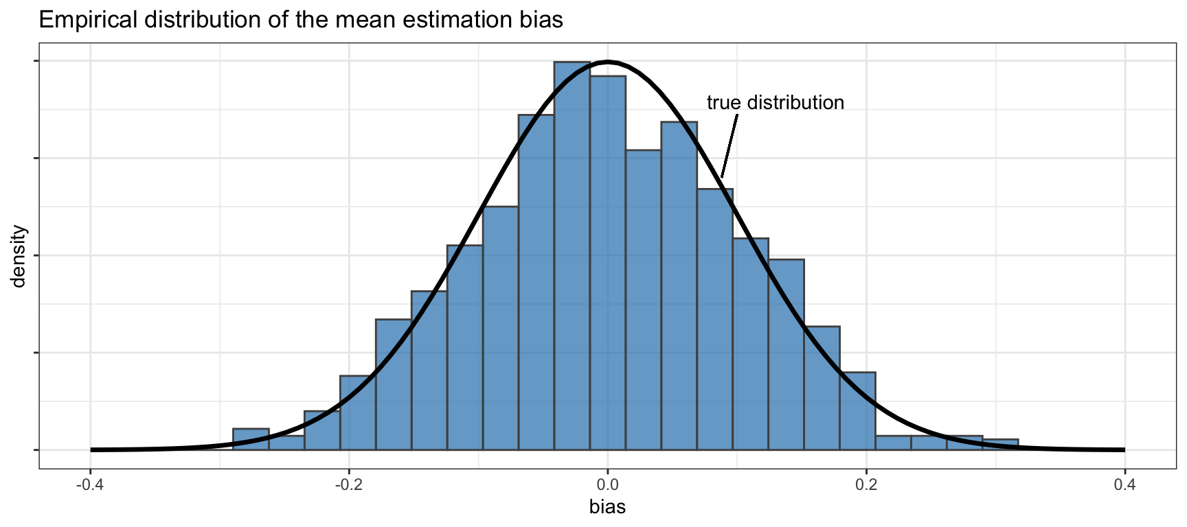
Figure 14.6: Empirical distribution of the sample mean bias via the bootstrap.
The Jackknife
The jackknife, proposed in the mid-1950s by M. Quenouille, is the precursor of the bootstrap. It was derived for estimating biases and standard errors of sample estimators. Given the \(n\) observations \(\bm{x}_1,\dots,\bm{x}_n\), the \(i\)th jackknife sample is obtained by removing the \(i\)th data point, \(\bm{x}_1,\dots,\bm{x}_{i-1},\bm{x}_{i+1},\dots,\bm{x}_n\). This effectively produces \(B=n\) bootstrap samples each with \(n-1\) observations. The jackknife can be shown to be an approximation to the bootstrap; more exactly, it makes a linear approximation to the bootstrap. Its accuracy depends on how “smooth” the estimator is; for highly nonlinear functions the jackknife can be inefficient, sometimes dangerously so.
Variations of the Bootstrap
A number of variations and extensions of the basic bootstrap have been proposed over the years. Some notable examples include:
Parametric bootstrap: The original bootstrap methodology mimics the true data distribution by sampling the observations with replacement. Thus, the procedure is distribution-independent or nonparametric. However, there are parametric versions of the bootstrap (Efron and Tibshirani, 1993). The idea is to make some assumption concerning the true data distribution (for example, assuming the family of Gaussian distributions), estimate the parameters of the distribution from the observed data, and then generate as much data as desired using that parametric distribution.
Block bootstrap: The basic bootstrap method breaks down when the data contains structural dependency. A variety of block bootstrap methods have been proposed to deal with dependent data (Lahiri, 1999).
Random subspace method: The random subspace method was proposed in the context of decision trees in order to decrease the correlation among trees and avoid overfitting (T. K. Ho, 1998). The idea is to let each learner use a randomly chosen subspace of the features. In fact, this was a key component in the development of random forests in machine learning.
Bag of little bootstraps: In order to deal with large data sets with a massive number of observations, the bag of little bootstraps was proposed incorporating features of both the bootstrap and subsampling to yield a robust, computationally efficient means of assessing the quality of estimators (Kleiner et al., 2014).
Bagging
The bootstrap is as a way of assessing the accuracy of a parameter estimate or a prediction; interestingly, it can also be used to improve the estimate or prediction itself. Bootstrap aggregating or the acronym bagging refers to a method for generating multiple versions of some estimator or predictor via the bootstrap and then using these to get an aggregated version (Breiman, 1996; Hastie et al., 2009). Bagging can improve the accuracy of the basic estimator or predictor, which typically suffers from sensitivity to the realization of the random data. Mathematically, bagging is a simple average of the bootstrap replicates: \[ \hat{\bm{\theta}}^{\textm{bag}} = \frac{1}{B}\sum_{b=1}^B \hat{\bm{\theta}}^{*(b)}. \]
14.3.2 Portfolio Resampling
In portfolio design, an optimization problem is formulated based on \(T\) observations of the assets’ returns, \(\bm{x}_1,\dots,\bm{x}_T\), whose solution is supposedly an optimal portfolio \(\w\). As previously discussed, this solution is very sensitive to the inherent noise in the observed data or in the noise in the estimated parameters used in the portfolio formulation, such as the mean vector \(\hat{\bmu}\) and covariance matrix \(\hat{\bSigma}\).
Fortunately, we can capitalize on the results from the past half-century in statistics; in particular, we can use resampling techniques, such as the bootstrap and bagging, to improve the portfolio design.
The idea of resampling was proposed in the 1990s as a way to assess the accuracy of designed portfolios. The naive approach consists of using the available data to design a series of mean–variance portfolios and then obtaining the efficient frontier, but this is totally unreliable due to the high sensitivity of these portfolios on the data realization (the computed efficient frontier is not realistic and not representative of new data). Instead, resampling allows the computation of a more reliable efficient frontier, called the resampled efficient frontier, as well as the identification of statistically equivalent portfolios (Jorion, 1992; Michaud and Michaud, 1998).
In the context of data with temporal structure (as happens with many econometrics time series), apart from block bootstrap methods, a maximum entropy bootstrap has been proposed (Vinod, 2006). This method can be applied not only to time series of returns but even directly to time series of prices, which clearly have a strong temporal structure.
Portfolio Bagging
The technique of aggregating portfolios was considered in 1998 via a bagging procedure (Michaud and Michaud, 1998, 2007, 2008; Scherer, 2002):
- Resample the original data \((\bm{x}_1,\dots,\bm{x}_T)\) \(B\) times via the bootstrap method and estimate \(B\) different versions of the mean vector and covariance matrix: \(\hat{\bmu}^{*(b)}\) and \(\hat{\bSigma}^{*(b)}\) for \(b=1,\dots,B\).
- Solve the optimal portfolio \(\w^{*(b)}\) for each bootstrap sample.
- Average the portfolios via bagging: \[ \w^{\textm{bag}} = \frac{1}{B}\sum_{b=1}^B \w^{*(b)}. \]
This bagging procedure for portfolio aggregation is simple, and the only bottleneck is the increase in computational cost by a factor of the number of bootstraps \(B\) compared to the naive approach.
Portfolio Subset Resampling
An attempt to reduce the computational cost of the portfolio bagging procedure is the subset resampling technique (Shen and Wang, 2017). The idea is to sample the asset dimension rather than the observation (temporal) dimension, which is the same technique used to develop random forests (T. K. Ho, 1998). In more detail, instead of using all the \(N\) assets, the method randomly selects a subset, for which a portfolio of reduced dimensionality can be designed, which translates into a reduced computational cost. A rule of thumb is to select subsets of \(\lceil N^{0.7} \rceil\) or \(\lceil N^{0.8} \rceil\) assets; for example, for \(N=50\) the size of the subsets would be of \(16\) or \(23\), respectively. This procedure is repeated a number of times to finally aggregate all the computed portfolios. Note that since the portfolios are of reduced dimensionality, zeros are implicitly used in the elements corresponding to the other dimensions prior to the averaging.
A side benefit from the subset resampling technique, apart from the reduced computational cost, is that the parameters are better estimated because the ratio of observations to dimensionality is automatically increased in a significant way (see Chapter 3 for details on parameter estimation). For example, suppose we have \(T=252\) daily observations; the nominal ratio for \(N=50\) assets would be \(T/N \approx 5\), whereas the ratio for subset resampling would be \(T/N^{0.7} \approx 16\) or \(T/N^{0.8} \approx 11\). Numerical experiments will confirm that this is a good technique in practice.
Portfolio Subset Bagging
Random subset resampling along the asset domain can be straightforwardly combined with the bootstrap along the temporal domain (Shen et al., 2019). In this case, each bootstrap sample only contains a subset of the \(N\) assets.
14.3.3 Numerical Experiments
The goal of portfolio resampling is in making the solution more stable and less sensitive to the errors in the parameter estimation, gaining in robustness compared to a naive design.
Sensitivity of Resampled Portfolios
The extreme sensitivity of the naive mean–variance portfolio was shown in Figure 14.1. Then, robust portfolio optimization was shown to be less sensitive in Figure 14.2. We now repeat the same numerical experiment with resampled portfolios to observe their sensitivity.
Figure 14.7 shows the sensitivity of a bagged portfolio with \(B=200\) bootstrap samples over six different realizations of the estimation error in the parameters. Compared to Figure 14.1, it is clear that bagging helps to produce more stable and less sensitive portfolios.
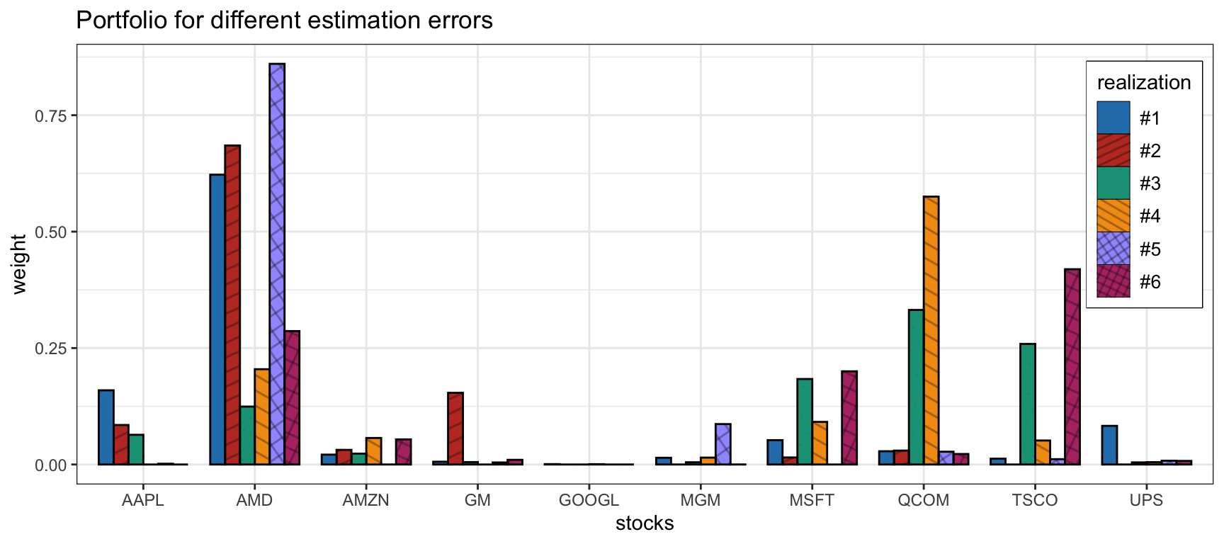
Figure 14.7: Sensitivity of the bagged mean–variance portfolio.
Comparison of Naive vs. Resampled Portfolios
Now that we have empirically observed the improved stability of mean–variance resampled portfolios, we can assess their performance in comparison with the naive design. In particular, we consider resampled portfolios via bagging, subset resampling, and subset bagging. Backtests are conducted for 50 randomly chosen stocks from the S&P 500 during 2017–2020.
Figure 14.8 shows the empirical distribution of the achieved mean–variance objective, as well as the Sharpe ratio, calculated over 1,000 Monte Carlo noisy observations. We can observe that resampled portfolios are more stable and do not suffer from extreme bad realizations (unlike the naive portfolio). However, the naive portfolio can be superior for some realizations.
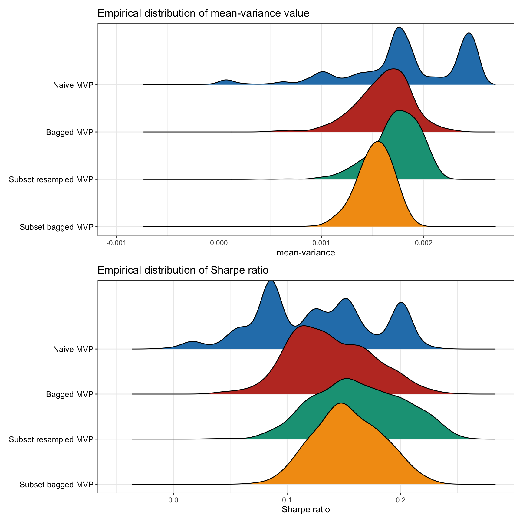
Figure 14.8: Empirical performance distribution of naive vs. resampled mean–variance portfolios.
Figure 14.9 shows the cumulative return and drawdown of the naive and resampled mean–variance portfolios for an illustrative backtest. We can observe how the resampled portfolios seem to be less noisy. However, this is just a single backtest and more exhaustive multiple backtests are necessary.
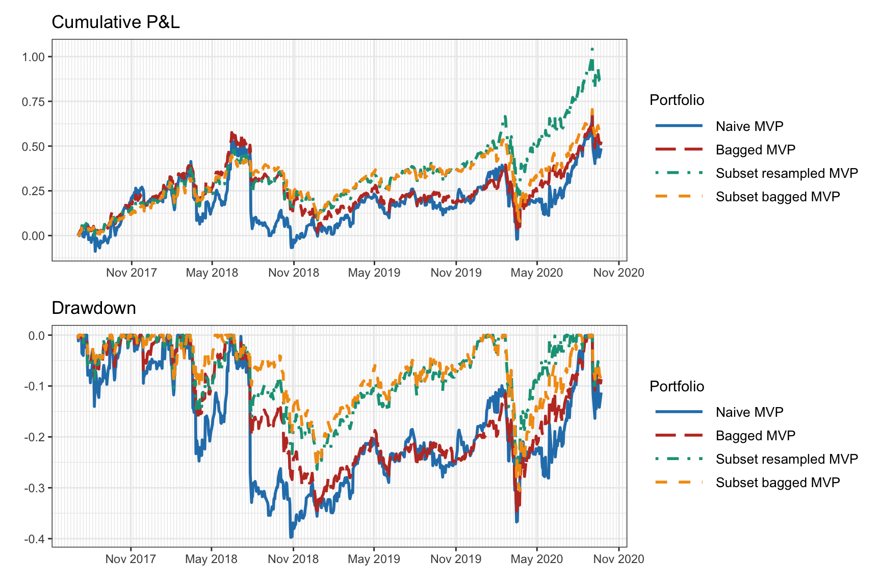
Figure 14.9: Backtest of naive vs. resampled mean–variance portfolios.
Finally, multiple backtests are conducted for 200 realizations of 50 randomly chosen stocks from the S&P 500 from random periods during 2015–2020. Figure 14.10 shows the results in terms of the Sharpe ratio and drawdown, confirming that the resampled portfolios are superior to the naive portfolio.
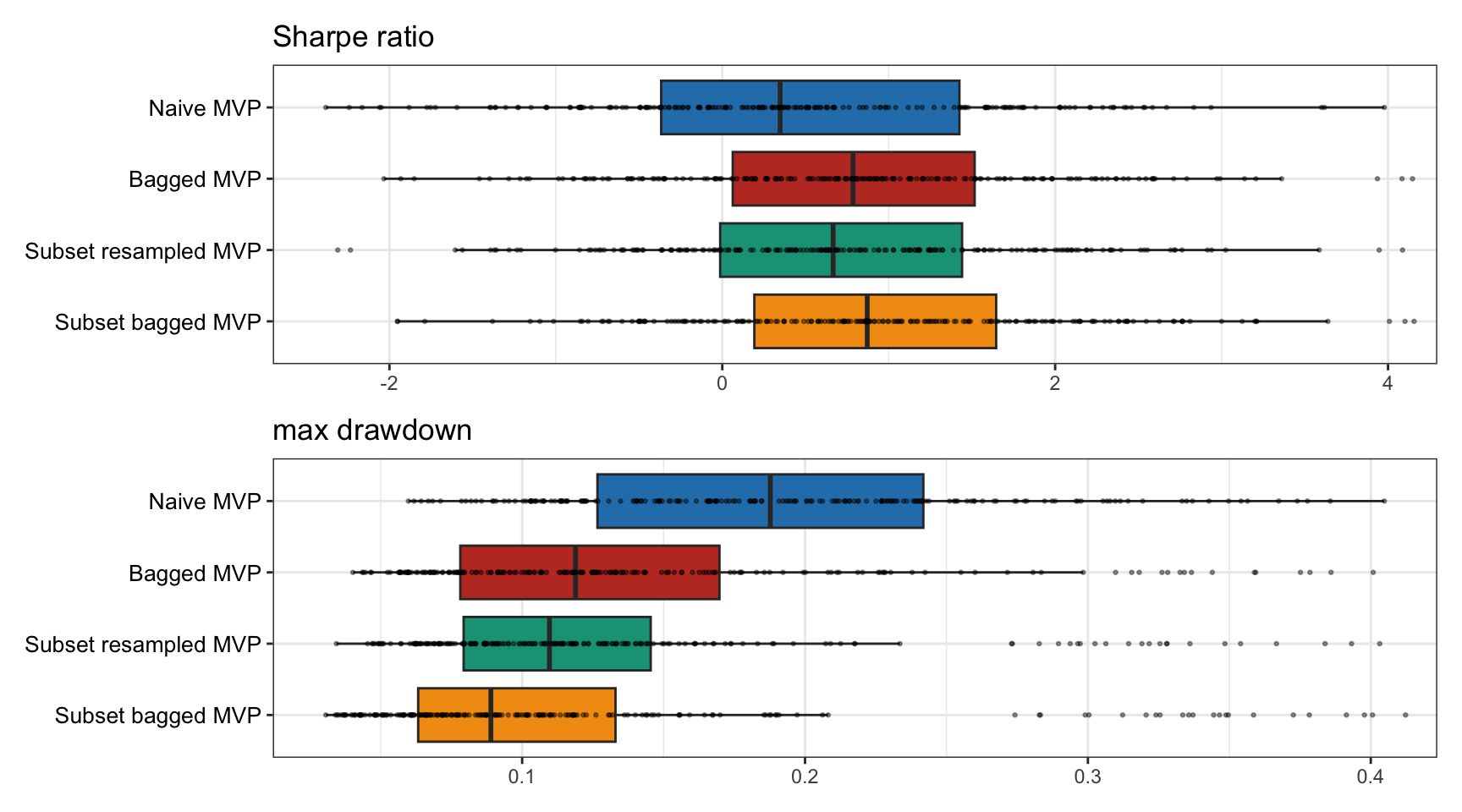
Figure 14.10: Multiple backtests of naive vs. resampled mean–variance portfolios.