B.9 Alternating Direction Method of Multipliers (ADMM)
The alternating direction method of multipliers (ADMM) is a practical algorithm that resembles BCD (see Section B.6), but is able to cope with coupled block variables in the constraints (recall that BCD requires each of the variable blocks to be independently constrained). For details, the reader is referred to Boyd et al. (2010) and Beck (2017).
Consider the convex optimization problem \[\begin{equation} \begin{array}{ll} \underset{\bm{x},\bm{z}}{\textm{minimize}} & f(\bm{x}) + g(\bm{z})\\ \textm{subject to} & \bm{A}\bm{x} + \bm{B}\bm{z} = \bm{c}, \end{array} \tag{B.14} \end{equation}\] where the variables \(\bm{x}\) and \(\bm{z}\) are coupled via the constraint \(\bm{A}\bm{x} + \bm{B}\bm{z} = \bm{c}.\) We are going to explore techniques to try to decouple the variables in order to derive simpler practical algorithms rather than attempting to solve (B.14) directly.
A first attempt to decouple the \(\bm{x}\) and \(\bm{z}\) in (B.14) is via the dual problem (see Section A.6 in Appendix A). More exactly, the dual ascent method updates the dual variable \(\bm{y}\) via a gradient method and, at each iteration, the Lagrangian is solved for the given \(\bm{y}\): \[ \begin{array}{ll} \underset{\bm{x},\bm{z}}{\textm{minimize}} & L(\bm{x},\bm{z}; \bm{y}) \triangleq f(\bm{x}) + g(\bm{z}) + \bm{y}^\T\left(\bm{A}\bm{x} + \bm{B}\bm{z} - \bm{c}\right), \end{array} \] which now clearly decouples into two separate problems over \(\bm{x}\) and \(\bm{z}\). This decoupling leads to the dual decomposition method, developed in the early 1960s, where the primal variables \(\bm{x}\) and \(\bm{z}\) are optimized in parallel: \[ \left. \begin{aligned} \bm{x}^{k+1} &= \underset{\bm{x}}{\textm{arg min}}\;\;f(\bm{x}) + (\bm{y}^k)^\T\bm{A}\bm{x}\\ \bm{z}^{k+1} &= \underset{\bm{z}}{\textm{arg min}}\;\;g(\bm{z}) + (\bm{y}^k)^\T\bm{B}\bm{z}\\ \bm{y}^{k+1} &= \bm{y}^{k} + \alpha^k \left(\bm{A}\bm{x}^{k+1} + \bm{B}\bm{z}^{k+1} - \bm{c}\right) \end{aligned} \quad \right\} \qquad k=0,1,2,\dots, \] where \(\alpha^k\) is the stepsize. This method is able to decouple the primal variables; however, it requires many technical assumptions to work and it is often slow.
A second attempt to solve problem (B.14) with fewer technical assumptions and with a faster algorithm is via the method of multipliers, developed in the late 1960s, which substitutes the Lagrangian by the augmented Lagrangian: \[ L_\rho(\bm{x},\bm{z}; \bm{y}) \triangleq f(\bm{x}) + g(\bm{z}) + \bm{y}^\T\left(\bm{A}\bm{x} + \bm{B}\bm{z} - \bm{c}\right) + \frac{\rho}{2}\|\bm{A}\bm{x} + \bm{B}\bm{z} - \bm{c}\|_2^2. \] The algorithm is then \[ \left. \begin{aligned} \left(\bm{x}^{k+1},\bm{z}^{k+1}\right) &= \underset{\bm{x},\bm{z}}{\textm{arg min}}\;\;L_\rho(\bm{x},\bm{z};\bm{y}^k)\\ \bm{y}^{k+1} &= \bm{y}^{k} + \rho \left(\bm{A}\bm{x}^{k+1} + \bm{B}\bm{z}^{k+1} - \bm{c}\right) \end{aligned} \quad \right\} \qquad k=0,1,2,\dots, \] where the penalty parameter \(\rho\) now serves as the (constant) stepsize. This method converges under much more relaxed conditions. Unfortunately, it cannot achieve decoupling in \(\bm{x}\) and \(\bm{z}\) because of the term \(\|\bm{A}\bm{x} + \bm{B}\bm{z} - \bm{c}\|_2^2\) in the augmented Lagrangian.
A third and final attempt is ADMM, proposed in the mid-1970s, which combines the good features of both the dual decomposition method and the method of multipliers. The idea is to minimize the augmented Lagrangian like in the method of multipliers, but instead of performing a joint minimization over \((\bm{x},\bm{z})\), a single round of the BCD method is performed (see Section B.6). This update follows an alternating or sequential fashion, which accounts for the name “alternating direction,” and leads to the ADMM iterations: \[ \left. \begin{aligned} \bm{x}^{k+1} &= \underset{\bm{x}}{\textm{arg min}}\;\; L_\rho(\bm{x},\bm{z}^k;\bm{y}^k)\\ \bm{z}^{k+1} &= \underset{\bm{z}}{\textm{arg min}}\;\; L_\rho(\bm{x}^{k+1},\bm{z};\bm{y}^k)\\ \bm{y}^{k+1} &= \bm{y}^{k} + \rho \left(\bm{A}\bm{x}^{k+1} + \bm{B}\bm{z}^{k+1} - \bm{c}\right) \end{aligned} \quad \right\} \qquad k=0,1,2,\dots \] This method successfully decouples the primal variables \(\bm{x}\) and \(\bm{z}\), while enjoying faster convergence with few technical conditions required for convergence.
For convenience, it is common to express the ADMM iterative updates in terms of the scaled dual variable \(\bm{u}^k = \bm{y}^k/\rho\) as used in Algorithm B.9.
Algorithm B.9: ADMM to solve the problem in (B.14).
Choose initial point \(\left(\bm{x}^0,\bm{z}^0\right)\) and \(\rho\);
Set \(k \gets 0\);
repeat
- Iterate primal and dual variables: \[ \begin{aligned} \bm{x}^{k+1} &= \underset{\bm{x}}{\textm{arg min}}\;\; f(\bm{x}) + \frac{\rho}{2}\left\|\bm{A}\bm{x} + \bm{B}\bm{z}^k - \bm{c} + \bm{u}^k\right\|_2^2,\\ \bm{z}^{k+1} &= \underset{\bm{z}}{\textm{arg min}}\;\; g(\bm{z}) + \frac{\rho}{2}\left\|\bm{A}\bm{x}^{k+1} + \bm{B}\bm{z} - \bm{c} + \bm{u}^k\right\|_2^2,\\ \bm{u}^{k+1} &= \bm{u}^{k} + \left(\bm{A}\bm{x}^{k+1} + \bm{B}\bm{z}^{k+1} - \bm{c}\right); \end{aligned} \]
- \(k \gets k+1\);
until convergence;
B.9.1 Convergence
Many convergence results for ADMM are discussed in the literature ((Boyd et al., 2010), and references therein). Theorem B.6 summarizes the most basic, but still very general, convergence result.
Theorem B.6 (Convergence of ADMM) Suppose that (i) the functions \(f(\bm{x})\) and \(g(\bm{z})\) are convex and both the \(\bm{x}\)-update and the \(\bm{z}\)-update are solvable, and (ii) the Lagrangian has a saddle point. Then, we have:
- residual convergence: \(\bm{A}\bm{x}^k + \bm{B}\bm{z}^k - \bm{c}\rightarrow\bm{0}\) as \(k\rightarrow\infty\), that is, the iterates approach feasibility;
- objective convergence: \(f(\bm{x}) + g(\bm{z})\rightarrow p^\star\) as \(k\rightarrow\infty\), that is, the objective function of the iterates approaches the optimal value; and
- dual variable convergence: \(\bm{y}^k\rightarrow\bm{y}^\star\) as \(k\rightarrow\infty\).
Note that \(\{\bm{x}^k\}\) and \(\{\bm{z}^k\}\) need not converge to optimal values, although such results can be shown under additional assumptions.
In practice, ADMM can be slow to converge to high accuracy. However, it is often the case that ADMM converges to modest accuracy within a few tens of iterations (depending on the specific application), which is often sufficient for many practical applications. This behavior is reminiscent of the gradient method (after all, the update of the dual variable is also a first-order method like gradient descent) and also different from the fast convergence of Newton’s method.
B.9.2 Illustrative Examples
We now give a few illustrative examples of applications of ADMM, along with numerical experiments.
Example B.12 (Constrained convex optimization) Consider the generic convex optimization problem \[ \begin{array}{ll} \underset{\bm{x}}{\textm{minimize}} & f(\bm{x})\\ \textm{subject to} & \bm{x} \in \mathcal{X}, \end{array} \] where \(f\) is convex and \(\mathcal{X}\) is a convex set.
We could naturally use an algorithm for solving constrained optimization problems. Interestingly, we can use ADMM to transform this problem into an unconstrained one. More specifically, we can employ ADMM by defining \(g\) to be the indicator function of the feasible set \(\mathcal{X}\), \[ g(\bm{x}) \triangleq \left\{\begin{array}{ll} 0 & \bm{x}\in\mathcal{X},\\ +\infty & \textm{otherwise}, \end{array}\right. \] and then formulating the equivalent problem \[ \begin{array}{ll} \underset{\bm{x},\bm{z}}{\textm{minimize}} & f(\bm{x}) + g(\bm{z})\\ \textm{subject to} & \bm{x} - \bm{z} = \bm{0}. \end{array} \] This produces the following ADMM algorithm: \[ \left. \begin{aligned} \bm{x}^{k+1} &= \underset{\bm{x}}{\textm{arg min}}\;\; f(\bm{x}) + \frac{\rho}{2}\left\|\bm{x} - \bm{z}^k + \bm{u}^k\right\|_2^2\\ \bm{z}^{k+1} &= \left[\bm{x}^{k+1} + \bm{u}^k\right]_\mathcal{X}\\ \bm{u}^{k+1} &= \bm{u}^{k} + \left(\bm{x}^{k+1} - \bm{z}^{k+1}\right) \end{aligned} \quad \right\} \qquad k=0,1,2,\dots, \] where \([\cdot]_\mathcal{X}\) denotes projection on the set \(\mathcal{X}\).
Example B.13 (\(\ell_2\)–\(\ell_1\)-norm minimization via ADMM) Consider the \(\ell_2\)–\(\ell_1\)-norm minimization problem \[ \begin{array}{ll} \underset{\bm{x}}{\textm{minimize}} & \frac{1}{2}\|\bm{A}\bm{x} - \bm{b}\|_2^2 + \lambda\|\bm{x}\|_1. \end{array} \] This problem can be conveniently solved via BCD (see Section B.6), MM (see Section B.7), SCA (see Section B.8), or simply by calling a QP solver. We will now develop a simple iterative algorithm based on ADMM that leverages the element-by-element closed-form solution.
We start by reformulating the problem as \[ \begin{array}{ll} \underset{\bm{x},\bm{z}}{\textm{minimize}} & \frac{1}{2}\|\bm{A}\bm{x} - \bm{b}\|_2^2 + \lambda\|\bm{z}\|_1\\ \textm{subject to} & \bm{x} - \bm{z} = \bm{0}. \end{array} \] The \(\bm{x}\)-update, given \(\bm{z}\) and the scaled dual variable \(\bm{u}\), is the solution to \[ \begin{array}{ll} \underset{\bm{x}}{\textm{minimize}} & \frac{1}{2}\|\bm{A}\bm{x} - \bm{b}\|_2^2 + \frac{\rho}{2}\left\|\bm{x} - \bm{z} + \bm{u}\right\|_2^2, \end{array} \] given by \(\bm{x}=\left(\bm{A}^\T\bm{A} + \rho\bm{I}\right)^{-1}\left(\bm{A}^\T\bm{b} +\rho(\bm{z} - \bm{u})\right)\), whereas the \(\bm{z}\)-update, given \(\bm{x}\) and \(\bm{u}\), is the solution to \[ \begin{array}{ll} \underset{\bm{z}}{\textm{minimize}} & \frac{\rho}{2}\left\|\bm{x} - \bm{z} + \bm{u}\right\|_2^2 + \lambda\|\bm{z}\|_1 \end{array} \] given by \(\bm{z} = \mathcal{S}_{\lambda/\rho} \left(\bm{x} + \bm{u}\right)\), where \(\mathcal{S}_{\lambda/\rho}(\cdot)\) is the soft-thresholding operator defined in (B.11).
Thus, the ADMM is finally given by the iterates \[ \left. \begin{aligned} \bm{x}^{k+1} &= \left(\bm{A}^\T\bm{A} + \rho\bm{I}\right)^{-1}\left(\bm{A}^\T\bm{b} +\rho\left(\bm{z}^k - \bm{u}^k\right)\right)\\ \bm{z}^{k+1} &= \mathcal{S}_{\lambda/\rho} \left(\bm{x}^{k+1} + \bm{u}^k\right)\\ \bm{u}^{k+1} &= \bm{u}^{k} + \left(\bm{x}^{k+1} - \bm{z}^{k+1}\right) \end{aligned} \quad \right\} \qquad k=0,1,2,\dots \] Figure B.13 shows the convergence of the ADMM iterates.
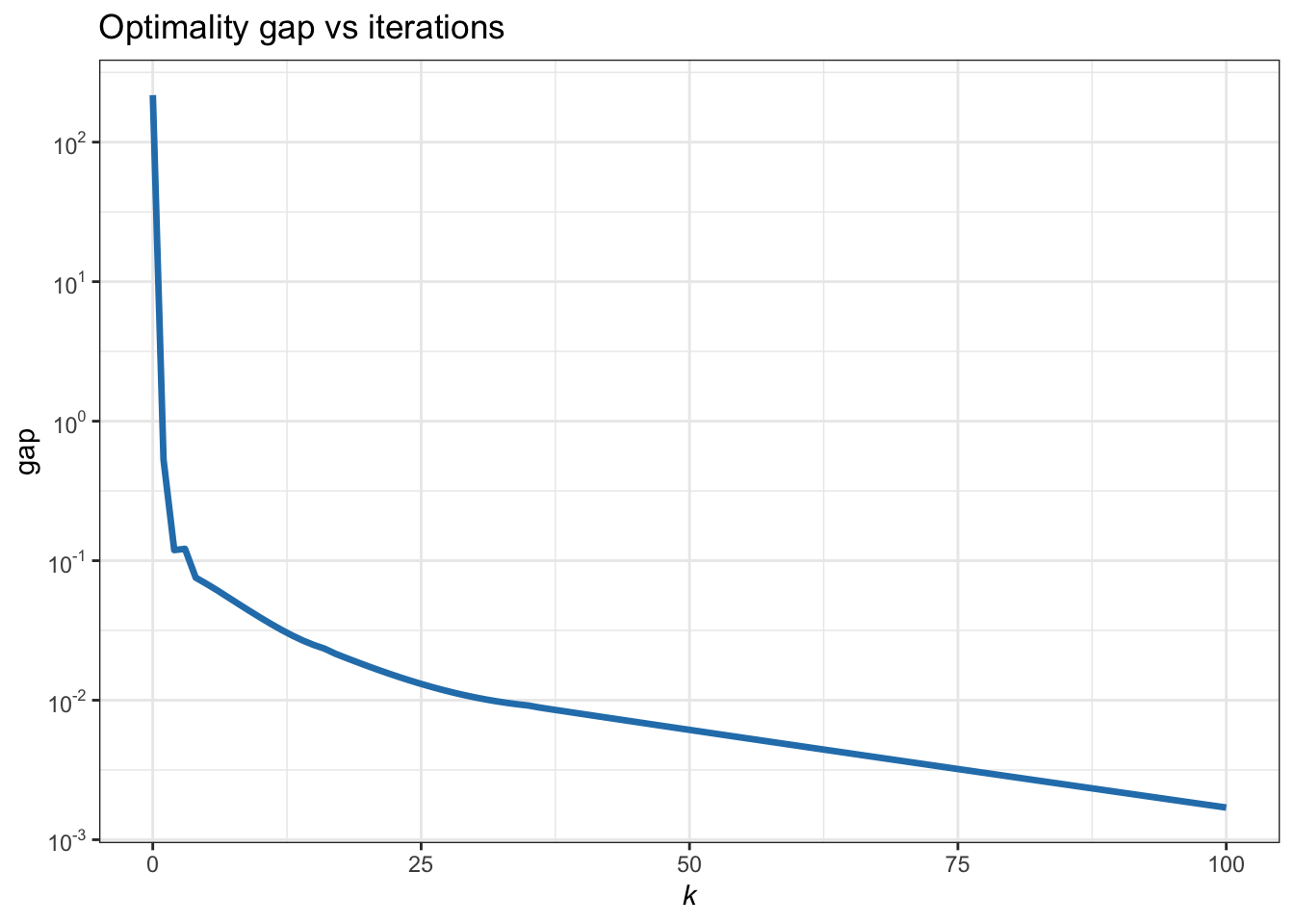
Figure B.13: Convergence of ADMM for the \(\ell_2\)–\(\ell_1\)-norm minimization.