8.4 Backtesting with Historical Market Data
As we have already discussed, a backtest evaluates the out-of-sample performance of an investment strategy using past observations. These observations can be used in a multitude of ways from the simplest method to more sophisticated versions.
One first classification is according to whether the past observations are used (i) directly to assess the historical performance as if the strategy had been run in the past (considered in detail in this section), or (ii) indirectly to simulate scenarios that did not happen in the past, such as stress tests (treated in the next section). Each approach has its pros and cons; in fact, both are useful and complement each other.
Assuming the historical data is used directly to assess the performance, we can further differentiate four types of backtest methods:
- vanilla (one-shot) backtest
- walk-forward backtest
- \(k\)-fold cross-validation backtest
- multiple randomized backtest.
The walk-forward backtest technique is so prevalent that, in fact, the term “backtest” has become a de facto synonym for walk-forward “historical simulation.” We now elaborate on these different approaches.
8.4.1 Vanilla Backtest
The simplest possible backtest, which we call a vanilla backtest, involves dividing the available data into in-sample data and out-of-sample data. The in-sample data is used to design the strategy and the out-of-sample to evaluate it. The reason we need two sets of data should be clear by now: if the same data is used to design the strategy and to evaluate it, we would obtain spectacular but unrealistic performance results that would not be representative of the future performance with new data (this is because the strategy would overfit the data).
The in-sample data is typically further divided into training data and cross-validation (CV) data, whereas the out-of-sample data is also called test data. The training data is used to fit the model, that is, to choose the parameters of the model, whereas the CV data is employed to choose the so-called hyper-parameters. Figure 8.9 illustrates the data split for this type of vanilla backtest. Additionally, one may leave some small gap in between the in-sample and out-of-sample data (to model the fact that one may not be able to execute the designed portfolio immediately).

Figure 8.9: Data split in a vanilla backtest.
As an illustrative example, one may divide the available data into 70% in-sample and 30% out-of-sample for testing. The in-sample data may be further divided into 70% for training and 30% for cross validation. The training data may be used, for instance, to estimate the mean vector \(\bmu\) and covariance matrix \(\bSigma\), whereas the CV data may be used to choose the hyper-parameter \(\lambda\) in the mean–variance portfolio formulation (see Section 7.1). One can simply try different values of \(\lambda\), say, 0.1, 0.5, 1.0, and 2.0, then evaluate the performance of each design with the CV data to choose the best-performing value of \(\lambda\). At this point, one can fit the model again (i.e., estimate \(\bmu\) and \(\bSigma\)) using all the in-sample data (i.e., training plus cross-validation data). Finally, one can use the test data to assess the performance of the designed portfolio.
The result of a vanilla backtest can be seen in Figure 8.10 in the form of cumulative P&L and drawdown of the portfolios, as well as in Table 8.2 in the form of numerical values of different performance measures over the whole period.
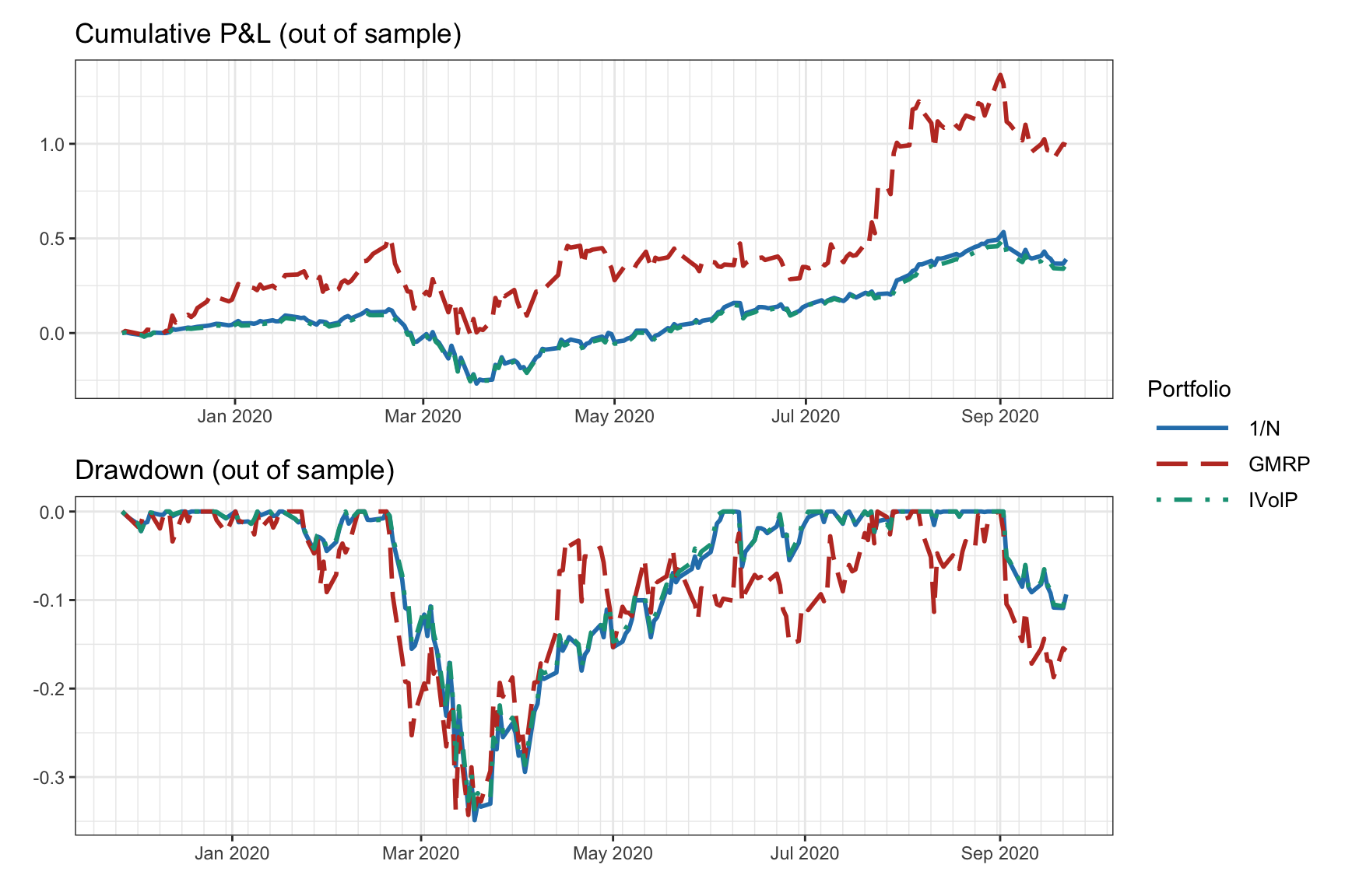
Figure 8.10: Vanilla backtest: cumulative P&L and drawdown.
| Portfolio | Sharpe ratio | Annual return | Annual volatility | Sortino ratio | Max drawdown | CVaR (0.95) |
|---|---|---|---|---|---|---|
| 1/\(N\) | 1.18 | 49% | 42% | 1.63 | 35% | 7% |
| GMRP | 1.62 | 105% | 65% | 2.58 | 34% | 9% |
| IVolP | 1.14 | 46% | 41% | 1.58 | 34% | 6% |
The vanilla backtest is widely used in academic publications, blogs, fund brochures, and so on. However, it has two main problems:
- A single backtest is performed, in the sense that a single historical path is evaluated.
- The execution of the backtest is not representative of the way it would have been conducted in real life, that is, the portfolio is designed once and kept fixed for the whole test period, whereas in real life as new data becomes available the portfolio is updated (this is precisely addressed by the walk-forward backtest).
8.4.2 Walk-Forward Backtest
The walk-forward backtest improves the vanilla backtest by redesigning the portfolio as new data becomes available, effectively mimicking the way it would be done in live trading. It is therefore a historical simulation of how the strategy would have performed in the past (its performance can be reconciled with paper trading). This is the most common backtest method in the financial literature (Pardo, 2008).
In signal processing, this is commonly referred to as implementation on a rolling-window or sliding-window basis. This means that at time \(t\) one will use a window of the past \(k\) samples \(t-k, \dots, t-1\), called the lookback window, as training data or in-sample data. As with the vanilla backtest, one can leave a gap between the last-used observation and the time in which the portfolio is executed (this is to be on the safe side and avoid potential issues, such as look-ahead bias). A variation of the rolling window is the so-called expanding window (also called anchored walk-forward backtest), by which at time \(t\) all the previous data is used, that is, all the samples \(1,2,\dots,t-1\) (the window is expanding with \(t\), hence the name).
Figure 8.11 illustrates the rolling-window split of data into in-sample and out-of-sample corresponding to a walk-forward backtest.

Figure 8.11: Data splitting in a rolling-window or walk-forward backtest.
The result of a walk-forward backtest with daily reoptimization can be seen in Figure 8.12 in the form of cumulative P&L and drawdown of the portfolios, as well as in Table 8.3 in the form of numerical values of different performance measures over the whole period.
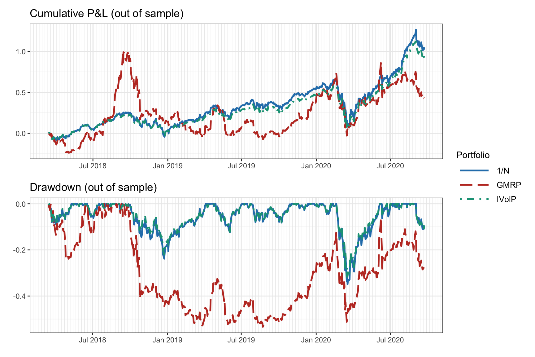
Figure 8.12: Walk-forward backtest: cumulative P&L and drawdown.
| Portfolio | Sharpe ratio | Annual return | Annual volatility | Sortino ratio | Max drawdown | CVaR (0.95) |
|---|---|---|---|---|---|---|
| 1/\(N\) | 1.10 | 33% | 30% | 1.54 | 35% | 5% |
| GMRP | 0.54 | 27% | 50% | 0.75 | 53% | 8% |
| IVolP | 1.09 | 31% | 28% | 1.52 | 32% | 4% |
Thus, the walk-forward backtest mimics the way live trading would be implemented and is the most common backtest method in finance. However, it still suffers from two critical issues:
- It still represents a single backtest, in the sense that a single historical path is evaluated (hence, the danger of overfitting).
- It is not uncommon to make some mistake with the time alignment and generate leakage (i.e., a form of look-ahead bias where future information leaks and is incorrectly used).
8.4.3 \(k\)-Fold Cross-Validation Backtest
The main drawback of the vanilla backtest and the walk-forward backtest is that a single historical path is evaluated. That is, in both cases a single backtest is performed. The idea in the \(k\)-fold cross-validation backtest is to test \(k\) alternative scenarios (of which only one corresponds to the historical sequence).
In fact, \(k\)-fold cross-validation is a common approach in machine learning (ML) applications (G. James et al., 2013), composed of the following steps:
- Partition the dataset into \(k\) subsets.
- For each subset \(i=1,\dots,k\):
- train the ML algorithm on all subsets excluding \(i\); and
- test the fitted ML algorithm on the subset \(i\).

Figure 8.13: Data splitting in a \(k\)-fold cross-validation backtest (with \(k=5\)).
Figure 8.13 illustrates the \(k\)-fold cross-validation split of data for \(k=5\). An implicit assumption in \(k\)-fold cross-validation is that the order of the blocks is irrelevant. This is true in many ML applications where the data is i.i.d. With financial data, however, this does not hold. While one may model the returns as uncorrelated, they are clearly not independent (e.g., the absolute values of the returns are highly correlated, as observed in Chapter 2, Figures 2.19–2.22).
In fact, leakage refers to situations when the training set contains information that also appears in the test set (it is a form of look-ahead bias). Some techniques can be employed to reduce the likelihood of leakage (López de Prado, 2018a). Nevertheless, due to the temporal structure in financial data, it is the author’s opinion that \(k\)-fold cross-validation backtests can be very dangerous in practice and are better avoided.
Summarizing, some of the issues with the \(k\)-fold cross-validation backtest include:
- It is still using a single path of data.
- It does not have a clear historical interpretation.
- Most importantly, leakage is possible (and likely) because the training data does not trail the test data.
8.4.4 Multiple Randomized Backtests
The main drawback of the vanilla and walk-forward backtests is that a single historical path is evaluated. The \(k\)-fold cross-validation backtest attempts to address this issue by testing \(k\) alternative scenarios; however, there is a significant problem with leakage and, in addition, only one of them corresponds to the historical sequence. With the multiple randomized backtest we can effectively deal with those issues in a satisfactory manner by generating a number of different backtests (each of them representing a different historical path) while respecting the order of training data followed by test data (to avoid leakage).
The basic idea of multiple randomized backtests is very simple:
- Start with a large amount of historical data (preferably large in time and in assets).
- Repeat \(k\) times:
- resample dataset: choose randomly a subset of the \(N\) available assets and a (contiguous) subset of the total period of time; and
- perform a walk-forward or rolling-window backtest of this resampled dataset.
- Collect statistics on the results of the \(k\) backtests.

Figure 8.14: Data splitting in multiple randomized backtests.
Figure 8.14 illustrates the data split in multiple randomized backtests. For example, if the data contains 500 stocks over a period of 10 years, one can resample the data by choosing, say, 200 randomly chosen stocks over random periods of 2 contiguous years. This will introduce some randomness in each individual dataset and it will span different market regimes encountered over the 10 years.
To illustrate multiple randomized backtests, we take a dataset of \(N=10\) stocks over the period 2017–2020 and generate 200 resamples each with \(N=8\) randomly selected stocks and a random period of two years. Then we perform a walk-forward backtest with a lookback window of one year, reoptimizing the portfolio every month.
Table 8.4 shows the backtest results in table form with different performance measures over the whole period. Figure 8.15 plots the barplots of the median values of maximum drawdown and annualized volatility (over the 200 individual backtests), whereas Figure 8.16 shows the boxplots of the Sharpe ratio and maximum drawdown. Clearly, the statistics on the multiple individual backtests provide a more accurate representation of the true capabilities of each portfolio. Nevertheless, it is still valid to say that this does not guarantee any future performance.
| Portfolio | Sharpe ratio | Annual return | Annual volatility | Sortino ratio | Max drawdown | CVaR (0.95) |
|---|---|---|---|---|---|---|
| 1/\(N\) | 1.01 | 28% | 25% | 1.42 | 25% | 4% |
| GMVP | 0.72 | 16% | 22% | 1.01 | 24% | 3% |
| IVolP | 0.94 | 24% | 23% | 1.33 | 23% | 3% |
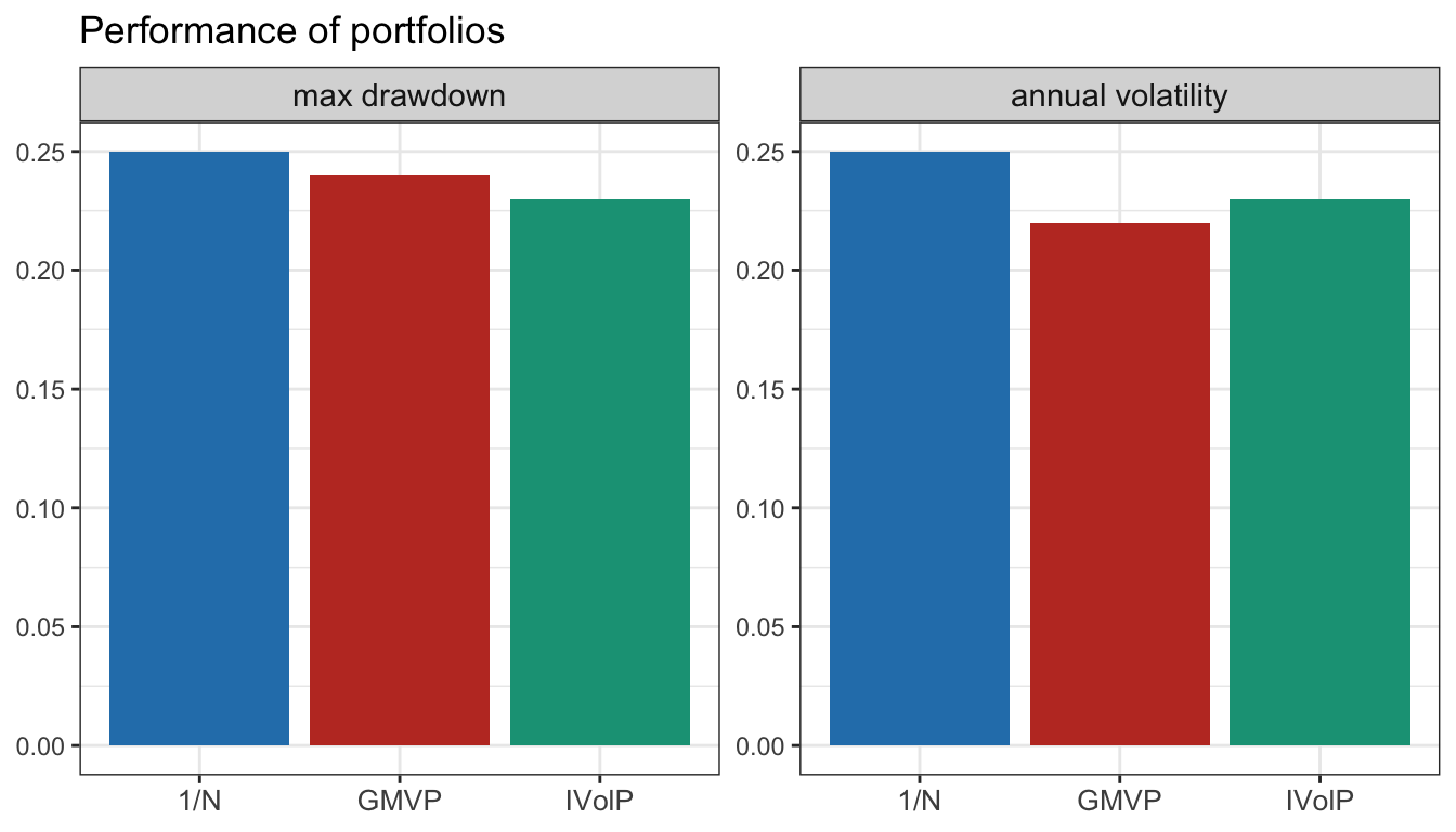
Figure 8.15: Multiple randomized backtests: barplots of maximum drawdown and annualized volatility.
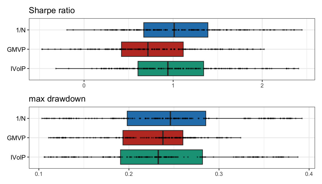
Figure 8.16: Multiple randomized backtests: boxplots of Sharpe ratio and maximum drawdown.
Multiple randomized backtests, while not perfect, seem to address the main drawbacks of the other types of backtests covered here. Therefore, in the author’s opinion, it is the preferred method for backtesting.