10.5 Drawdown Portfolios
Drawdown portfolios can be approached via statistical modeling of the returns based on dynamic programming (Cvitanic and Karatzas, 1995; Grossman and Zhou, 1993), as well as from a more data-driven perspective based on a sample-path (realization) of portfolio returns (Chekhlov et al., 2004), as we consider here.
As we know, the return of a portfolio \(\w\) at time \(t\) is given by \(R_t = \w^\T\bm{r}_t\), where \(\bm{r}_t\) denotes linear returns or approximately log-returns. However, since the drawdown is derived from the cumulative return, we need the portfolio cumulative return: \[ R_t^\textm{cum} = \w^\T\bm{r}_t^\textm{cum}, \] where the cumulative returns of the assets can be computed as \[ \bm{r}_t^\textm{cum} = \sum_{\tau=1}^t \bm{r}_\tau. \] Depending on whether we use linear or log-returns in \(\bm{r}_t\), this expression corresponds to the uncompounded linear returns or compounded log-returns, respectively (see Section 6.1.3 in Chapter 6 for details). Note that the value of the portfolio is \(1 + R_t^\textm{cum}\).
The absolute drawdown is \[ D_t(\w) = \underset{1 \le \tau \le t}{\textm{max}} \; \w^\T\bm{r}_\tau^\textm{cum} - \w^\T\bm{r}_t^\textm{cum} \] and a constraint of the form \(D_t(\w) \le \alpha\) can be written as the linear (after adding some dummy variables) constraint \[ \w^\T\bm{r}_t^\textm{cum} \ge \underset{1 \le \tau \le t}{\textm{max}} \; \w^\T\bm{r}_\tau^\textm{cum} - \alpha. \]
Similarly, the normalized drawdown is \[ \bar{D}_t(\w) = \frac{\underset{1 \le \tau \le t}{\textm{max}} \; \w^\T\bm{r}_\tau^\textm{cum} - \w^\T\bm{r}_t^\textm{cum}}{1+\underset{1 \le \tau \le t}{\textm{max}} \; \w^\T\bm{r}_\tau^\textm{cum}} \] and a constraint of the form \(\bar{D}_t(\w) \le \alpha\) can be written as the linear (again after adding some dummy variables) constraint \[ \w^\T\bm{r}_t^\textm{cum} \ge (1-\alpha) \; \underset{1 \le \tau \le t}{\textm{max}} \; \w^\T\bm{r}_\tau^\textm{cum} - \alpha. \]
10.5.1 Formulation for the Max-DD Portfolio
The mean–Max-DD formulation replaces the usual variance term \(\w^\T\bSigma\w\) by the maximum drawdown as a measure of risk: \[\begin{equation} \begin{array}{ll} \underset{\w}{\textm{maximize}} & \w^\T\bmu - \lambda \, \textm{Max-DD}(\w)\\ \textm{subject to} & \w \in \mathcal{W}. \end{array} \tag{10.14} \end{equation}\] As usual, this problem can be similarly formulated by moving either the expected return or the risk term to the constraints (see Chapter 7).
Substituting for \(\textm{Max-DD}(\w) = \underset{1\le t\le T}{\textm{max}} D_t(\w)\), where \(D_t(\w)\) is the drawdown at time \(t\), leads to the problem \[ \begin{array}{ll} \underset{\w}{\textm{maximize}} & \w^\T\bmu - \lambda \, \underset{1\le t\le T}{\textm{max}} \left\{\underset{1 \le \tau \le t}{\textm{max}} \; \w^\T\bm{r}_\tau^\textm{cum} - \w^\T\bm{r}_t^\textm{cum}\right\}\\ \textm{subject to} & \w \in \mathcal{W}, \end{array} \] which is convex (assuming \(\mathcal{W}\) is convex) because the maximum of convex functions is convex (see Appendix A for details on convexity).
Writing the problem in epigraph form and introducing the auxiliary variables \(s\) and \(\bm{u}\) (\(u_0\triangleq-\infty\)) to get rid of the max operators leads to \[\begin{equation} \begin{array}{ll} \underset{\w, \bm{u}, s}{\textm{maximize}} & \begin{array}{l} \w^\T\bmu - \lambda \, s \end{array}\\ \textm{subject to} & \begin{array}[t]{ll} \w^\T\bm{r}_t^\textm{cum} \le u_t \le s + \w^\T\bm{r}_t^\textm{cum}, & \quad t=1,\dots,T,\\ u_{t-1} \le u_t,\\ \w \in \mathcal{W}, \end{array} \end{array} \tag{10.15} \end{equation}\] which is a linear program (assuming \(\mathcal{W}\) only contains linear constraints).
It is important to remark that, by definition, the worst drawdown is given by a single data point, which makes this risk measure extremely sensitive. In other words, minute changes in the portfolio weights and the specific time period examined (recall that the drawdown is path-dependent) may produce totally different values of the maximum drawdown. This makes this measure of risk not very reliable, which can be mitigated by using instead the average drawdown or the conditional drawdown-at-risk considered next. As an alternative, if the distribution is close to Gaussian, then the mean–variance framework may be sufficient (see Chapter 7), whereas if the distribution shows some skewness and heavy tails, then high-order portfolios can be used (see Chapter 9).
10.5.2 Formulation for the Ave-DD Portfolio
We can repeat the same procedure with the average drawdown instead: \[ \begin{array}{ll} \underset{\w}{\textm{maximize}} & \begin{aligned} \w^\T\bmu - \lambda \, \frac{1}{T}\sum_{t=1}^T \left(\underset{1 \le \tau \le t}{\textm{max}} \; \w^\T\bm{r}_\tau^\textm{cum} - \w^\T\bm{r}_t^\textm{cum}\right)\end{aligned}\\ \textm{subject to} & \w \in \mathcal{W}, \end{array} \] which is also convex (assuming \(\mathcal{W}\) is convex) because the maximum of convex functions is convex (see Appendix A for details on convexity).
Writing the problem in epigraph form and introducing the auxiliary variables \(s\) and \(\bm{u}\) (\(u_0\triangleq-\infty\)) to get rid of the max operator leads to \[\begin{equation} \begin{array}{ll} \underset{\w, \bm{u}, s}{\textm{maximize}} & \begin{array}{l} \w^\T\bmu - \lambda \, s \end{array}\\ \textm{subject to} & \frac{1}{T}\sum_{t=1}^T u_t \le \frac{1}{T}\sum_{t=1}^T\w^\T\bm{r}_t^\textm{cum} + s,\\ & \w^\T\bm{r}_t^\textm{cum} \le u_t, \qquad t=1,\dots,T,\\ & u_{t-1} \le u_t,\\ & \w \in \mathcal{W}, \end{array} \tag{10.16} \end{equation}\] which is a linear program (assuming \(\mathcal{W}\) only contains linear constraints).
10.5.3 Formulation for the CVaR-DD Portfolio
To formulate the mean–CVaR-DD portfolio, we will make use of the following variational convex representation of the CVaR-DD (or CDaR) (Chekhlov et al., 2004, 2005): \[ \textm{CVaR-DD}(\w) = \underset{\tau}{\textm{inf}} \left\{\tau + \frac{1}{1-\alpha}\frac{1}{T}\sum_{t=1}^T\left(D_t(\w) - \tau\right)^+\right\}. \]
This leads to the mean–CVaR-DD formulation: \[ \begin{array}{ll} \underset{\w, \tau}{\textm{maximize}} & \begin{aligned} \w^\T\bmu - \lambda \left(\tau + \frac{1}{1-\alpha}\frac{1}{T}\sum_{t=1}^T\left(\underset{1 \le \tau \le t}{\textm{max}} \; \w^\T\bm{r}_\tau^\textm{cum} - \w^\T\bm{r}_t^\textm{cum} - \tau\right)^+\right) \end{aligned}\\ \textm{subject to} & \w \in \mathcal{W}, \end{array} \] where the auxiliary variable \(\tau\) has been conveniently moved from the inner minimization to the outer maximization. This problem is convex, assuming that \(\mathcal{W}\) is a convex set.
After a series of manipulations to get rid of the nondifferentiable max operator and \((\cdot)^+\), and the introduction of the auxiliary variables \(s\), \(\bm{z}\), and \(\bm{u}\) (\(u_0\triangleq-\infty\)), the problem can be finally rewritten as \[\begin{equation} \begin{array}{ll} \underset{\w, \tau, s, \bm{z}, \bm{u}}{\textm{maximize}} & \w^\T\bmu - \lambda \, s\\ \textm{subject to} & s \ge \tau + \frac{1}{1-\alpha}\frac{1}{T}\sum_{t=1}^T z_t,\\ & 0 \le z_t \ge u_t - \w^\T\bm{r}_t^\textm{cum} - \tau, \qquad t=1,\dots,T,\\ & \w^\T\bm{r}_t^\textm{cum} \le u_t,\\ & u_{t-1} \le u_t,\\ & \w \in \mathcal{W}, \end{array} \tag{10.17} \end{equation}\] which is a linear program (assuming \(\mathcal{W}\) only contains linear constraints).
Similarly to the EVaR portfolio in (10.11)–(10.12), one can easily formulate a drawdown EVaR simply by replacing in (10.12) the loss terms \(-\w^\T\bm{r}_t\) by \(D_t(\w)=\underset{1 \le \tau \le t}{\textm{max}} \; \w^\T\bm{r}_\tau^\textm{cum} - \w^\T\bm{r}_t^\textm{cum}\).
10.5.4 Numerical Experiments
We now compare several drawdown-based portfolios, namely, that based on the minimization of the maximum drawdown formulated in (10.15), the average drawdown formulated in (10.16), and the drawdown CVaR formulated in (10.17). To focus on the effect of the risk measure, we ignore the expected return term in the optimization (effectively letting \(\lambda\rightarrow\infty\)) and also include the GMVP as a reference benchmark.
Similarly to the CVaR portfolios, a word of caution is necessary here. The problem boils down to the fact that the worst drawdowns happen with low probability, which translates into very few samples being used in the computation of the risk measure. This is specially true for the maximum drawdown (a single sample) and the drawdown CVaR (extremely few samples).
Figure 10.7 shows boxplots of the Sharpe ratio and maximum drawdown for 200 realizations of 50 randomly chosen stocks, from the S&P 500 during 2015–2020, reoptimizing the portfolios every month with a lookback of one year. The drawdown portfolios do not seem to outperform the simple GMVP benchmark, although more exhaustive empirical experiments would be necessary.
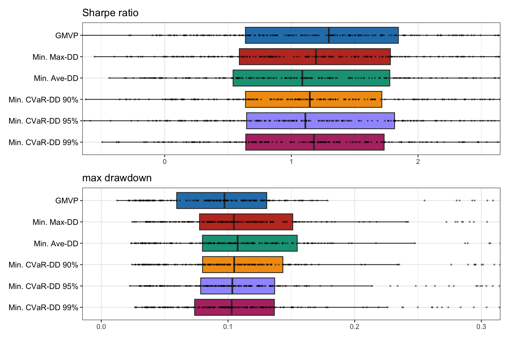
Figure 10.7: Backtest performance of drawdown portfolios.