8.2 The Seven Sins of Quantitative Investing
In 2005, a practitioner report compiled the “Seven Sins of Fund Management” (Montier, 2005) (of which sins #1 and #5 are the most directly related to backtesting):
- Sin #1: Forecasting (Pride)
- Sin #2: The illusion of knowledge (Gluttony)
- Sin #3: Meeting companies (Lust)
- Sin #4: Thinking you can out-smart everyone else (Envy)
- Sin #5: Short time horizons and overtrading (Avarice)
- Sin #6: Believing everything you read (Sloth)
- Sin #7: Group-based decisions (Wrath).
In 2014, a team of quants at Deutsche Bank published a study under the suggestive title “Seven Sins of Quantitative Investing” (Luo et al., 2014). These seven sins are a few basic backtesting errors that most journal publications make routinely:
- Sin #1: Survivorship bias
- Sin #2: Look-ahead bias
- Sin #3: Storytelling bias
- Sin #4: Overfitting and data snooping bias
- Sin #5: Turnover and transaction cost
- Sin #6: Outliers
- Sin #7: Asymmetric pattern and shorting cost.
In the following we will go over these seven sins of quantitative investing with illustrative examples.
8.2.1 Sin #1: Survivorship Bias
Survivorship bias is one of the common mistakes investors tend to make. Most people are aware of this bias, but few understand its significance.
Practitioners tend to backtest investment strategies using only those companies that are currently in business and still performing well, most likely listed in some index, such as the S&P 500 stock index. By doing that, they are ignoring stocks that have left the investment universe due to bankruptcy, delisting, being acquired, or simply underperforming the index.
In simple words, survivorship bias happens when you do not take into account stocks that you know in advance will not perform well in the future of the backtest period. Similarly, simply removing stocks from the universe because they have missing values in their data may have a misleading effect.
In fact, most available databases suffer from survivorship bias. In this context, the Center for Research in Security Prices (CRSP)41 maintains a comprehensive database of historical stock market data that is considered highly reliable and accurate, making it a valuable resource for those studying finance and investment. CRSP is widely used by academic researchers and financial professionals for conducting empirical research, analyzing historical stock market trends, and developing investment strategies. Figure 8.2 shows the effect of survivorship bias on the \(1/N\) portfolio on the S&P 500 stocks over several years.
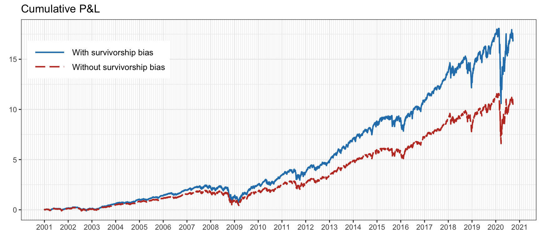
Figure 8.2: Effect of survivorship bias on the S&P 500 stocks.
Interestingly, the concept of survivorship bias does not happen uniquely in financial investment; it is rather a persistent phenomenon in many other areas. An illustrative example is that of modern-day billionaires who dropped out of college and went on to become highly successful (e.g., Bill Gates and Mark Zuckerberg). These few success stories distort people’s perceptions because they ignore the majority of college dropouts who are not billionaires.
8.2.2 Sin #2: Look-Ahead Bias
Look-ahead bias is the bias created by using information or data that were unknown or unavailable at the time when the backtesting was conducted. It is a very common bias in backtesting.
An obvious example of look-ahead bias lies in companies’ financial statement data. One has to be certain about the timestamp for each data point and take into account release dates, distribution delays, and backfill corrections.
A less conspicuous example of look-ahead bias comes from coding errors. This may happen, for instance, when training the parameters of a system using future information or simply when data is pre-processed with statistics collected from the whole block of data. Another common error comes from time alignment errors in the backtesting code. In more detail, computing the portfolio return as \(R^\textm{portf}_t = \w_{t}^\T\bm{r}_t\) would be totally incorrect (see (6.4) for the correct expression) since the design of the portfolio \(\w_{t}\) used information up to time \(t\) and the returns \(\bm{r}_t = (\bm{p}_t - \bm{p}_{t-1})\oslash\bm{p}_{t-1}\) implicitly assume that the position was executed at time \(t-1\) (of course this argument becomes invalid if the portfolio \(\w_{t}\) is assumed to use information only up to \(t-1\), or if the returns are defined with a time lag as \(\bm{r}_t = (\bm{p}_{t+1} - \bm{p}_{t})\oslash\bm{p}_{t}\)). An illustration of this issue can be found in Glabadanidis (2015) as explained in Zakamulin (2018), where the seemingly amazing performance of a strategy based on moving-average indicators vanishes completely under a proper backtest.
Figure 8.3 illustrates the effect of look-ahead bias (from a time alignment mistake when computing the returns) when trading a single stock with a simple strategy based on a moving average (to be exact, buying when the price is above the moving average of the past 10 values).
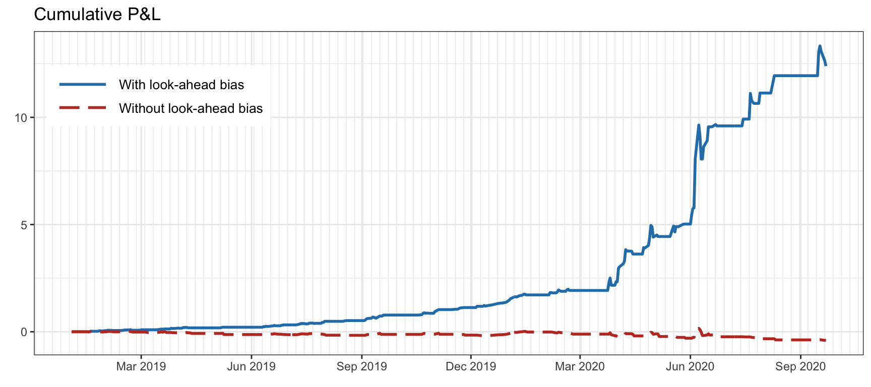
Figure 8.3: Effect of look-ahead bias (from a time alignment mistake) trading a single stock.
8.2.3 Sin #3: Storytelling Bias
We all love stories. It is believed that storytelling played a key role in the evolution of the human species. In fact, most bestselling popular science books are based on anecdotal stories, which may or may not have a corresponding solid statistical foundation. This is simply because they appeal to the general public, while statistics do not. Indeed, one of the most important ways to leave a deep impression with your audience is to tell stories rather than simply repeating facts and numbers.
Storytelling bias in financial data (or any other type of data, for that matter) happens when we make up a story ex post (i.e., after the observation of a particular event) to justify some random pattern. This is related to confirmation bias, which consists of favoring information that supports one’s pre-existing beliefs and ignoring contradicting evidence. Storytelling is pervasive in financial news, where supposed “experts” can justify any random pattern after the fact.
The antidote to storytelling bias is the collection of more historical data to see if the story passes a statistical test or the test of time. Unfortunately, in contrast to fields like physics, economics and finance have a limited number of observations, which hinders the resolution of storytelling bias.
Figure 8.4 illustrates the effect of story-telling bias by trading a single stock with a position indicated by a random binary sequence (which might have been generated by “Paul the Octopus”42). Before August 2018 one could be inclined to believe the story that the random sequence was a good predictor of the stock trend; however, eventually, when more data is collected, one has to come to the inevitable conclusion that it was a fluke.
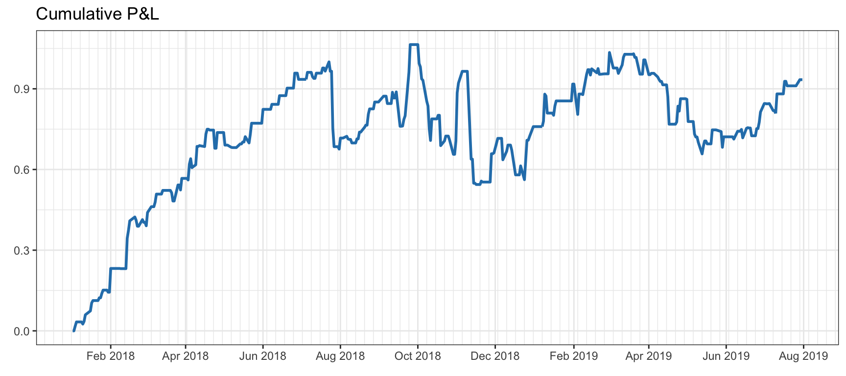
Figure 8.4: Effect of story-telling bias in the form of a random strategy that performs amazingly well until August 2018, but not afterwards.
8.2.4 Sin #4: Overfitting and Data Snooping Bias
In the fields of computer science and statistics, data mining refers to the computational process of discovering patterns in large data sets, often involving sophisticated statistical techniques, computation algorithms, and large-scale database systems. In principle, there is nothing negative about data mining. In finance, however, it often means manipulating data or models to find the desired pattern that an analyst wants to show.
Data snooping bias in finance (also loosely referred to as data mining bias) refers to the behavior of extensively searching for patterns or rules so that a model fits the data perfectly. Analysts often fine tune the parameters of their models and choose the ones that perform well in the backtesting. This is also referred to as overfitting in the machine learning literature.
With enough data manipulation, one can almost always find a model that performs very well on that data. This is why it is standard practice to split the data into in-sample and out-of-sample data: the in-sample data is used to estimate or train the model and design the portfolio, whereas the out-of-sample data is used to evaluate and test the portfolio. They are also referred to as training data and test data, respectively.
With the separation of data into training data and test data, it seems we should be safe; unfortunately, this is not the case. It is almost inevitable for the person or team researching a strategy to iterate the process by which the strategy under design is evaluated with the test data and then some adjustments are performed on the strategy. This is a vicious cycle that leads to catastrophic results. By doing that, the test data has inadvertently been used too many times and it has effectively become part of the training data. Unfortunately, this happens in almost all the publications to the point that one cannot trust published results: “Most backtests published in journals are flawed, as the result of selection bias on multiple tests” (López de Prado, 2018a).
In other words, looking long and hard enough at a given dataset will often reveal one or more models that seems promising but are in fact spurious (White, 2000).
One piece of advice that may help avoid overfitting is to avoid fine tuning the parameters (Chan, 2008). Even better, one could perform a sensitivity analysis on the parameters. That is, if a small change in some parameter affects the performance drastically, it is an indication that the strategy is too sensitive and lacks robustness. A sensitive strategy is dangerous because one cannot assess the future behavior with new data with any degree of confidence.
An illustrative example, provided in Arnott et al. (2019), shows a strategy with an impressive backtest result, only to reveal that the strategy is a preposterous long–short quintile portfolio that goes long on the stocks with an “S” on the third letter of the ticker symbol and goes short on the ones with the letter “U”.
Data snooping bias or overfitting is probably the most difficult bias to deal with. The ultimate test after a strategy or portfolio has been designed is to trade it with new data. This can be done in three different levels of accuracy: (i) simply wait to collect new data and then perform a proper backtest; (ii) use paper trading offered by most brokers, which consists of a realistic trading simulation without real money; and (iii) trade with real money, that is, live trading, albeit typically starting with a small budget.
Figure 8.5 illustrates the effect of data snooping or overfitting by trading a single stock with a strategy based on machine learning. In particular, a linear return forecast with a lookback window of 10 values is trained in two scenarios: using only the training data (as it should be) and using the training + test data (obviously, this produces overfitting). The overfitted backtest seems to indicate prediction power in the out of sample, whereas the reality could not be further from the truth.
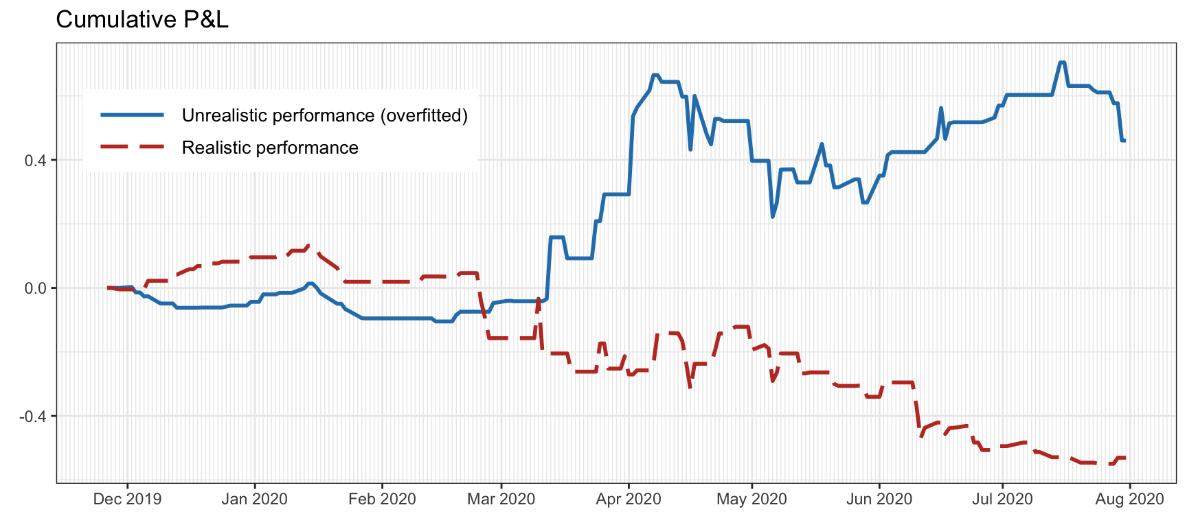
Figure 8.5: Effect of data snooping or overfitting on a backtest after tweaking the strategy too many times.
8.2.5 Sin #5: Turnover and Transaction Cost
Backtesting is often conducted in an ideal world: no transaction cost, no turnover constraint, unlimited long and short availability, and perfect liquidity. In reality, all investors are limited by some constraints. We now focus on the turnover and the associated transaction cost.
Turnover refers to the overall amount of orders to be executed when rebalancing the portfolio from \(\w_t\) to \(\w_{t}^\textm{reb}\), and is calculated as \(\|\w_{t}^\textm{reb} - \w_{t}\|_1\). As a first approximation, the transaction costs can be modeled as proportional to the turnover (see Section 6.1.4 for details). However, if the liquidity is not enough compared to the size of the turnover, then slippage may have a significant effect. This becomes more relevant as the rebalancing frequency increases. In the limit, simulating the transaction cost at the level of the limit order book can be extremely challenging and the only way to be certain about the cost incurred is to actually trade.
Figure 8.6 illustrates the detrimental effect of transaction costs on the daily-rebalanced inverse volatility portfolio on the S&P 500 stocks with fees of 60 bps. The effect of transaction costs slowly accumulates over time.
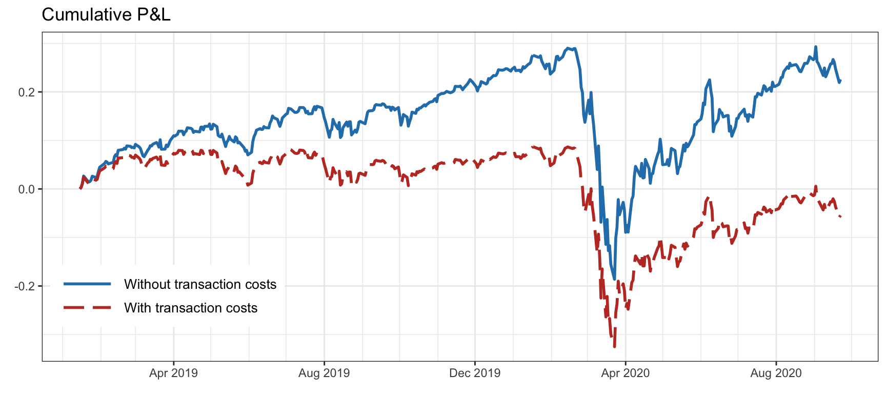
Figure 8.6: Effect of transaction costs on a portfolio (with daily rebalancing and fees of 60 bps).
The overall transaction cost depends on the turnover per rebalancing and the rebalancing frequency. Portfolios with a high rebalancing frequency are more prone to have an overall large turnover, which translates into high transaction costs. To be on the safe side, either the rebalancing frequency should be kept to a minimum or the turnover per rebalancing should be controlled (see Section 6.1.5). Nevertheless, having too slow a rebalancing frequency may lead to a portfolio that fails to adapt to the changing signal. Thus, deciding the rebalancing frequency of a strategy is a critical step in practice (see Section 6.1.5 in Chapter 6 for details).
8.2.6 Sin #6: Outliers
Outliers are events that do not fit the normal and expected behavior. They are not too uncommon in financial data and they can happen due to different reasons. Some outliers reflect a reality that actually happened due to some historical event. Others may be an artifact of the data itself, perhaps due to a momentaneous lack of liquidity of the market, or an abnormally large execution order, or even some error in the data.
In principle, outliers cannot be predicted and one can only try to be robust to them; this is why robust estimation methods (as in Chapter 3) and robust portfolio techniques (as in Chapter 14) are important in practice.
The danger when it comes to backtesting is to accidentally benefit from a few outliers, because that would distort the realistic assessment of a portfolio. More often than not, outliers are caused by data errors or specific events that are unlikely to be repeated in the future. Thus, one should not base the success of a portfolio on a few historical outliers, as the future performance will then rely on the realization of similar outliers. How should we then treat outliers in the historical data?
One way to deal with outliers is to control them so that they do not distort the backtest results. Traditional outlier control techniques include: winsorization (capping data at certain percentiles) and truncation/trimming/censoring (removing outliers from data sample). The data normalization process is closely related to outlier control.
Another way to deal with outliers is to keep the outliers, but making sure the potential success of the backtested strategies does not rely on them (unless one is actually trying to design a strategy solely based on outliers).
Figure 8.7 illustrates the effect of outlier control in the design phase of a quintile portfolio with hourly cryptocurrency data. In this case, outliers are removed if they are larger than 5% (recall these are hourly returns).
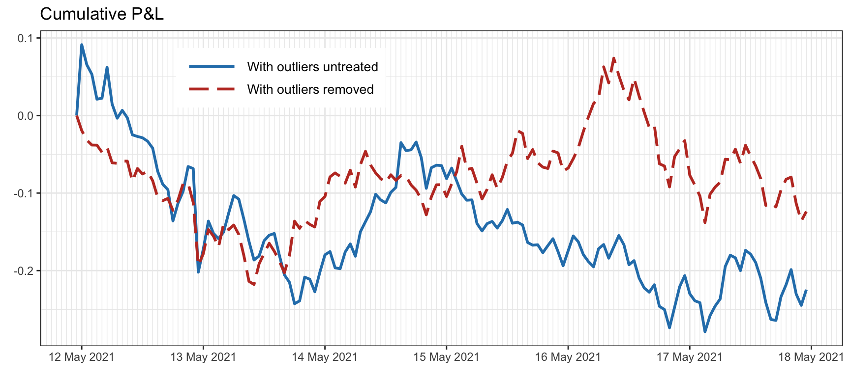
Figure 8.7: Effect of outliers on a backtest with hourly cryptocurrency data.
8.2.7 Sin #7: Asymmetric Pattern and Shorting Cost
In typical backtesting, analysts generally assume they can short any stocks at no cost or at the same level of cost. However, we need to be aware that borrowing cost can be prohibitively high for some stocks, while on other occasions, it could be impossible to locate the borrowing. For certain stocks, industries, or countries, there could also be government or exchange imposed rules that prohibit any shorting at all. Indeed, some countries do not allow short selling at all, while others limit its extent.43
For example, in the US market, during the 2008 global financial crisis period borrowing costs sky-rocketed – some financial stocks were even banned from being shorted, reflected by higher percentages of expensive-to-borrow stocks during this episode.
Interestingly, the effect of short availability not only affects backtests of portfolios that actually short sell but long positions may also suffer from the so-called “limited arbitrage” argument, by which arbitrageurs are prevented from immediately forcing prices to fair values.
How much difference would it make if we cannot short those hard-to-borrow stocks? Figure 8.8 shows the performance of two long–short quintile portfolios: an unrealistic portfolio that can perfectly long and short the top 20% and bottom 20% of the stocks, respectively, and a more realistic portfolio where only some easy-to-borrow stocks can actually be shorted (the definition of easy-to-borrow stocks used herein is a bit loose for illustration purposes).

Figure 8.8: Effect of shorting availability in a long–short quintile portfolio.
References
Paul the Octopus was a common octopus used to predict the results of association football matches. Accurate predictions in the 2010 World Cup brought him worldwide attention as an animal oracle. https://en.wikipedia.org/wiki/Paul_the_Octopus↩︎
In China, as of 2021, regulators only allow investors to short a portion of stocks traded on the Shanghai and Shenzhen stock exchanges. The list of stocks changes regularly and typically only includes companies with good fundamentals.↩︎