15.2 Cointegration and Correlation
Mean reversion, as previously described, refers to the tendency of a time series to return to its long-term average value over time. This property allows for a simple trading strategy: buy when below the average and sell when above. While it is virtually impossible to find an asset with controlled and predictable mean reversion, it is much easier to discover pairs of assets with a combined mean reversion property.
15.2.1 Cointegration
Cointegration refers to a property by which two (or more) assets, while not being mean reverting individually, may be mean reverting with respect to each other (Chan, 2013; Ehrman, 2006; Vidyamurthy, 2004). This commonly happens when the series themselves contain stochastic trends (i.e., they are nonstationary) but nevertheless they move closely together over time in a way that their difference remains stable (i.e., stationary). Thus, the concept of cointegration mimics the existence of a long-run equilibrium to which an economic system converges over time.
The intuitive idea is that, while it may be difficult or impossible to predict individual assets, it may be easier to predict their relative behavior. The typical example used to illustrate the concept of cointegration is that of a drunken man wandering the streets (random walk) with a dog (illustrated in Figure 15.3). Both paths of man and dog are nonstationary and difficult to predict, but the distance between them is mean reverting and stationary.

Figure 15.3: Random walk by a drunken man with a dog.
Mathematically, a multivariate time series, \(\bm{y}_1,\bm{y}_2,\bm{y}_3,\dots\), is cointegrated if some linear combination becomes integrated of lower order, for example, if \(\bm{y}_t\) is not stationary but the linear combination \(\w^\T\bm{y}_t\) is stationary for some weights \(\w\). In this sense, cointegration can be thought of as a more refined version of a time series being integrated of order 1. To be more specific, suppose the multivariate time series \(\bm{y}_t\) denotes the log-prices of some stocks. Such a time series is nonstationary (random walk) but after differencing we obtain the log-returns, which are stationary. Cointegration provides a more refined version that allows us to obtain a stationary time series without having to difference it. Instead, by taking a linear combination \(\w^\T\bm{y}_t\) we might be able to obtain a stationary time series. As covered later, this property has remarkable consequences in terms of trading and it forms the basics of pairs trading.
A simple and common way to model cointegration of two time series is as \[\begin{equation} \begin{aligned} y_{1t} &= \gamma \, x_{t} + w_{1t},\\ y_{2t} &= x_{t} + w_{2t}, \end{aligned} \tag{15.1} \end{equation}\] where \(x_t\) is a stochastic common trend defined as a random walk, \[ x_{t} = x_{t-1} + w_{t}, \] and the terms \(w_{1t}\), \(w_{2t}\), \(w_{t}\) are i.i.d. residual terms, mutually independent, with variances \(\sigma_1^2\), \(\sigma_2^2\), and \(\sigma^2\), respectively. The coefficient \(\gamma\) is the key quantity that determines the cointegration relationship. It is important to note that each of the time series, \(y_{1t}\) and \(y_{2t}\), is a random walk plus additional noise, therefore nonstationary. However, since they share a common stochastic trend, a simple linear combination of the two can eliminate this trend. The so-called spread is precisely this linear combination without the trend: \[ z_{t} = y_{1t} - \gamma \, y_{2t} = w_{1t} - \gamma \, w_{2t}, \] which is stationary and mean reverting.
15.2.2 Correlation
Correlation is a basic concept in probability that refers to how “related” two random variables are. We can use this measure for stationary time series but definitely not with nonstationary time series. In fact, when we refer to correlation between two financial assets, we are actually employing this concept on the returns of the assets and not the price values.
Specifically, given two time series of log-prices, \(y_{1t}\) and \(y_{2t}\), we can obtain the log-returns as the differences \(\Delta y_{1t}\) and \(\Delta y_{2t}\). Then the correlation can be safely defined, assuming stationarity, as \[ \rho = \frac{\E\left[\left(\Delta y_{1t} - \mu_1\right) \cdot \left(\Delta y_{2t} - \mu_2\right)\right]}{\sqrt{\textm{Var}(\Delta y_{1t}) \cdot \textm{Var}(\Delta y_{2t})}}, \] where \(\mu_1\) and \(\mu_2\) denote the means of \(\Delta y_{1t}\) and \(\Delta y_{2t}\), respectively, and the denominator normalizes with respect to the variances of the two variables, \(\textm{Var}(\Delta y_{1t})\) and \(\textm{Var}(\Delta y_{1t})\), so that the correlation is bounded as \(-1 \le \rho \le 1\).
The interpretation of correlation is quite simple: it is high when the two time series co-move (they move simultaneously in the same direction) and it is zero when they move independently.
15.2.3 Correlation vs. Cointegration
At this point, the concepts of correlation and cointegration have been introduced, but their similarity and difference may be unclear and confusing. After all, it seems that they both try to capture the concept of similarity of movements of two time series, so superficially they may seem to be similar concepts. However, they are totally different right from their definition.
As a matter of fact, the correlation of the differences of the two cointegrated time series in the model (15.1) can be analytically derived as \[ \rho = \frac{1}{\sqrt{1+2\frac{\sigma_{1}^{2}}{\sigma^{2}}}\sqrt{1+2\frac{\sigma_{2}^{2}}{\sigma^{2}}}}, \] which can be made as small as desired by properly choosing the variances of the residual terms \(\sigma_1^2\), \(\sigma_2^2\), and \(\sigma^2\). That is, we can have two perfectly cointegrated time series with an arbitrarily small correlation, which may be surprising at first. This reveals that cointegration and correlation are two totally different concepts, yet they both attempt to measure the similarity of the movements of two time series. The following examples illustrate this difference.
Consider the common trend model in (15.1) with \(\gamma=1\) and the standard deviations \(\sigma=0.1\) and \(\sigma_1=\sigma_2=0.2\). The theoretical correlation is \(\rho=\) 0.111, whereas the empirical correlation computed with 200 observations is \(\rho=0.034\), and with \(2\,000\) observations \(\rho=0.108\). Figure 15.4 shows the two nonstationary time series, \(y_{1t}\) and \(y_{2t}\), the stationary spread, \(z_{t}\), as well as the scatter plot of the differences \(\Delta y_{1t}\) vs. \(\Delta y_{2t}\), which does not show any preferred direction as expected for low correlation.
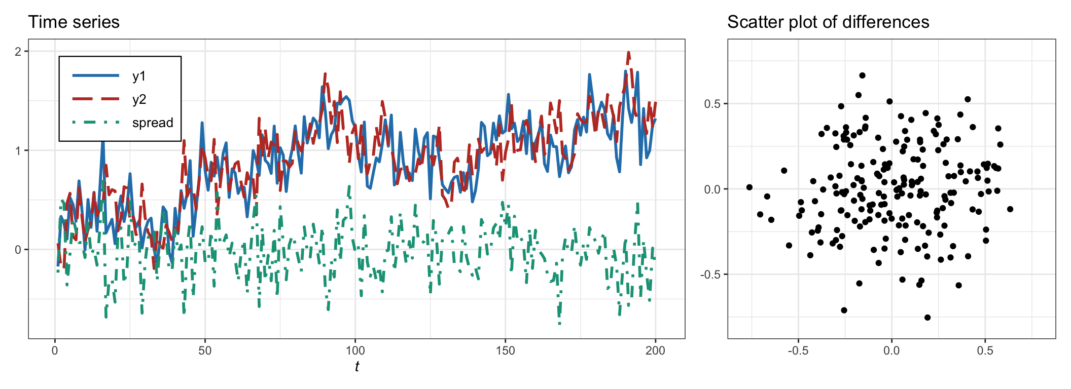
Figure 15.4: Example of cointegrated time series with low correlation.
Consider the common trend model in (15.1) with \(\gamma=1\) and the standard deviations \(\sigma=0.3\) and \(\sigma_1=\sigma_2=0.05\). In addition, add the linear trend \(0.01\times t\) to the first time series \(y_{1t}\), which will destroy the cointegration between the two time series while not affecting the correlation. In this case, the theoretical correlation is \(\rho=\) 0.947, whereas the empirical correlation computed with 200 observations is \(\rho=0.952\), and with \(2\,000\) observations \(\rho=0.941\). Figure 15.5 shows the two nonstationary time series, \(y_{1t}\) and \(y_{2t}\), the nonstationary spread, \(z_{t}\), as well as the scatter plot of the differences \(\Delta y_{1t}\) vs. \(\Delta y_{2t}\), which clearly shows a preferred direction as expected for high correlation.
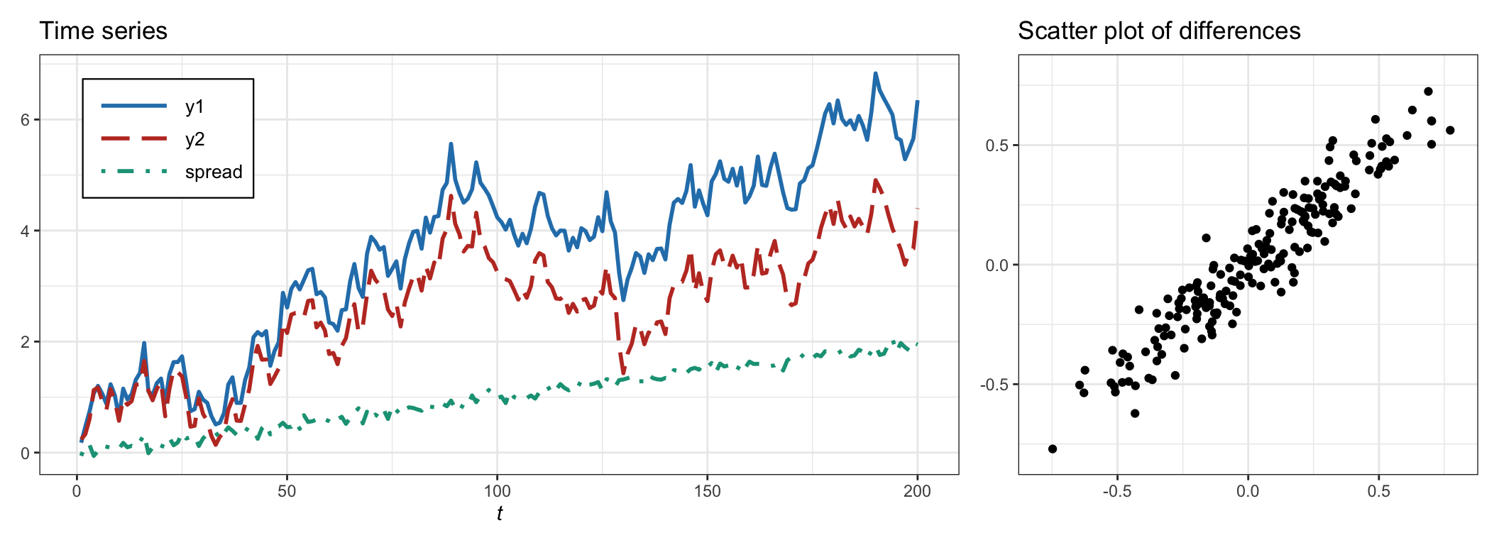
Figure 15.5: Example of non-cointegrated time series with high correlation.
Thus, both correlation and cointegration attempt to measure the same concept of co-movement of time series, but they do it in very different ways, namely:
Correlation is high when the two time series co-move (they move simultaneously in the same direction) and zero when they move independently.
Cointegration is high when the two time series move together and remain close to each other, and nonexistent when they do not stay together.
One way to understand the fundamental difference is in terms of short term vs. long term. Correlation is concerned with the short-term movements, that is, the directional movement from one period to the next, while ignoring the long-term trends. Cointegration, on the other hand, focuses on the long term, that is, whether the two time series have diverged or not after many periods, while being oblivious to short-term variations.
This short term vs. long term interpretation can be made more precise as follows. Define the difference of a time series \(y_{t}\) over \(k\) periods as \(r_t(k) = y_{t} - y_{t-k}\). Our goal is to measure the similarity of two time series \(y_{1t}\) and \(y_{2t}\) over \(t=0,\dots,T\):
Correlation does it via the one-period differences \(r_{1t}(1) = \Delta y_{1t}\) and \(r_{2t}(1) = \Delta y_{2t}\) over \(t=1,\dots,T\).
Cointegration measures the difference between the two time series \(y_{1t} - y_{2t}\) (assuming \(\gamma=1\) for simplicity). Equivalently, each time series can be shifted with its initial value and then they can be compared for divergence. Interestingly, these shifted time series are precisely the \(t\)-period differences \(r_{1t}(t) = y_{1t} - y_{10}\) and \(r_{2t}(t) = y_{2t} - y_{20}\) over \(t=1,\dots,T\).
For pairs trading, it is the cointegration that matters, and not the correlation, because the focus is precisely on the long-term mean reversion property.