15.5 Trading the Spread
Suppose we have discovered a cointegrated pair of log-price time series, \(y_{1t}\) and \(y_{2t}\), and have formed the spread \(y_{1t} - \gamma \, y_{2t},\) which is effectively using the two-asset portfolio \(\w = \left[1, -\gamma\right]^\T\) with a leverage of \(\| \w\|_1 = 1+\gamma\). In order to make fair comparisons, it is necessary to normalize the leverage to 1. Thus, the portfolio with normalized leverage is \[\begin{equation} \w = \frac{1}{1+\gamma}\begin{bmatrix} \;\;\;1\\ -\gamma \end{bmatrix}, \tag{15.2} \end{equation}\] with corresponding normalized spread \(z_{t} = \w^\T\bm{y}_{t}\). The return of this portfolio at time \(t\) (ignoring transaction costs) is given by \(\w^\T \left( \bm{y}_{t} - \bm{y}_{t-1} \right) = z_{t} - z_{t-1}\) (see Chapter 6 for details on portfolio notation). Suppose we enter a position at time \(t\) and after \(k\) periods the spread reverts to the mean and the position is closed. This would lead to a difference of at least \(|z_{t+k} - z_{t}| \ge s_0\), which is the portfolio return during these \(k\) periods.
Trading the spread boils down to deciding when to buy or short-sell the spread, and how much to invest (termed sizing). This is conveniently done by defining a “signal” time series \(s_1, s_2, s_3,\dots\), where \(s_t\) denotes the sizing (positive for buying, zero for no position, and negative for short-selling) usually bounded as \(-1 \le s_t \le 1\) to control the leverage. We will assume that the value of the signal at time \(t,\) \(s_t,\) has been decided based on information up to (and including) time \(t\), that is, \(\dots,\bm{y}_{t-2},\bm{y}_{t-1},\bm{y}_{t}\). Thus, the combination of the spread portfolio (15.2) and the signal \(s_t\) produces the time-varying portfolio \(s_t \times \w\), with corresponding return \[ R^\textm{portf}_t = s_{t-1} \times \w^\T \left( \bm{y}_{t} - \bm{y}_{t-1} \right) = s_{t-1} \times (z_{t} - z_{t-1}). \]
15.5.1 Trading Strategies
To define a strategy to trade the spread, it suffices to determine a rule for the sizing signal \(s_t\). For this purpose, it is convenient to use a normalized version of the spread, called the standard score or \(z\)-score: \[ z^\textm{score}_t = \frac{z_t - \E[z_t]}{\sqrt{\textm{Var}(z_t)}}, \] which has zero mean and unit variance. This \(z\)-score cannot be used in a real implementation since it is not causal and suffers from look-ahead bias (when estimating the mean and variance). A naive approach would be to use some training data to determine the mean and standard deviation, and then apply that to the future out-of-sample data. A more sophisticated way is to make the calculation adaptive by implementing it in a rolling fashion, for example via the so-called Bollinger Bands.
Bollinger Bands are a technical trading tool created by John Bollinger in the early 1980s. They arose from the need for adaptive trading bands and the observation that volatility was dynamic. They are computed on a rolling-window basis over some lookback window. In particular, the rolling mean and rolling standard deviation are first computed, from which the upper and lower bands are easily obtained (typically the mean plus/minus one or two standard deviations). In the context of the \(z\)-score, the spread can be adaptively normalized with the rolling mean and rolling standard deviation.
We now describe two of the simplest possible strategies for trading a spread, namely, the linear strategy and the thresholded strategy.
The linear strategy is very simple to describe based on the contrarian idea of buying low and selling high (Chan, 2013). As a first attempt, we could define the sizing signal simply as the negative \(z\)-score, \(s_t = -z^\textm{score}_t\), to gradually scale-in and scale-out or, even better, including a scaling factor as \(s_t = -z^\textm{score}_t / s_0\), where \(s_0\) denotes the threshold at which the signal is fully leveraged. In practice, to limit the leverage to 1, we can project this value to lie in the interval \([-1,1]\): \[ s_t = -\left[\frac{z^\textm{score}_t}{s_0}\right]_{-1}^{+1}, \] where \([\cdot]_a^b\) clips the argument to \(a\) if below that value and to \(b\) if above that value.
The thresholded strategy follows similarly the contrarian nature of buying low and selling high, but rather than linear it takes an all-in or all-out sizing based on thresholds (Vidyamurthy, 2004). The simplest implementation is based on comparing the \(z\)-score to a threshold \(s_0\): buy when the \(z\)-score is below \(-s_0\) and short-sell when it is above \(s_0\), while unwinding the position after reverting to the equilibrium value of zero. In terms of the sizing signal: \[ s_t = \begin{cases} \begin{aligned} +1 &\qquad \textm{if } z^\textm{score}_t < - s_0,\\ 0 &\qquad \textm{after }z^\textm{score}_t\textm{ reverts to }0,\\ -1 &\qquad \textm{if } z^\textm{score}_t > + s_0. \end{aligned} \end{cases} \]
Figures 15.13 and 15.14 illustrate the linear and thresholded strategies, respectively, based on a synthetic spread generated as an AR(1) with an autoregressive coefficient of 0.7. Observe the different nature of the sizing signal: continuous vs. on–off. The thresholds have been chosen arbitrarily as \(s_0=1\) and should be properly optimized for maximizing the profit (as described in detail in the next section). In practice, the rolling version of the \(z\)-score should be used to make it implementable without look-ahead bias, such as based on the Bollinger Bands (Chan, 2013).
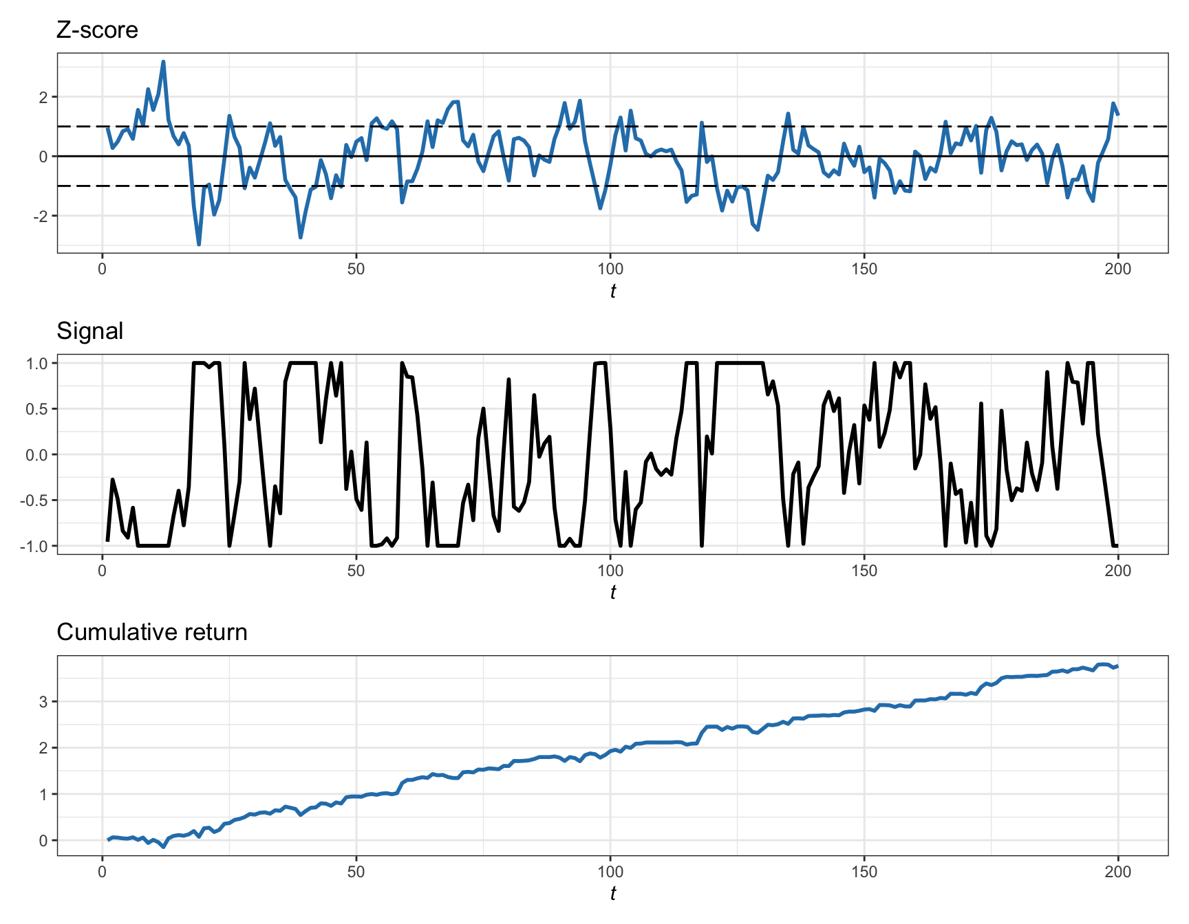
Figure 15.13: Illustration of pairs trading via the linear strategy on the spread.
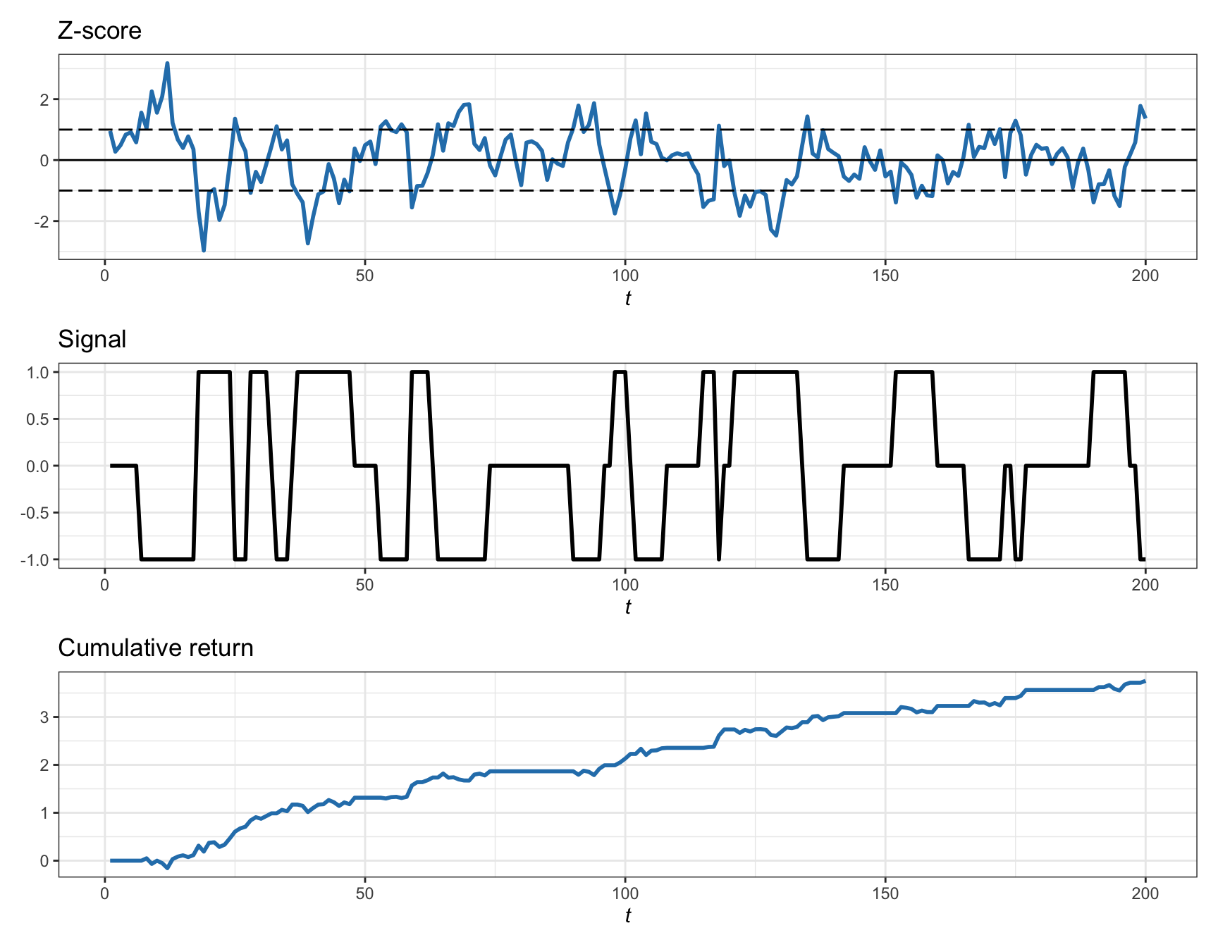
Figure 15.14: Illustration of pairs trading via the thresholded strategy on the spread.
15.5.2 Optimizing the Threshold
Consider now the simple thresholded strategy that buys when the \(z\)-score is below the threshold \(-s_0\) and short-sells when it is above \(s_0\), unwinding the position after reverting to the equilibrium value of zero. Note that in terms of the spread, the threshold is \(s_0 \times \sigma\), where \(\sigma\) is the standard deviation of the spread.
The choice of this threshold is critical as it determines how often the position is closed (cashing a profit) as well as how large that minimum profit is. The total profit equals the number of trades times the profit of each trade. Recall that, when a position is closed after \(k\) periods, the meaning of the spread difference \(z_{t+k} - z_t\) depends on whether the spread represents log-prices or prices:
- for log-prices, the spread difference denotes the log-return of the profit;
- for prices, the spread difference denotes the absolute profit (to be scaled with the initial budget).
Thus, after \(N^\textm{trades}\) successful trades have been executed, the total (uncompounded) profit can be accounted as \(N^\textm{trades} \times \sigma\, s_0\) (the compounded profit could also be used).
We will now obtain the optimum choice of the threshold to maximize the total profit in both parametric and nonparametric approaches.
Parametric Approach
Suppose the \(z\)-score follows a standard normal distribution, \(z^\textm{score}_t \sim \mathcal{N}(0,1)\). Then, the probability that it deviates from zero by \(s_0\) or more is \(1 - \Phi(s_{0})\), where \(\Phi(\cdot)\) is the cumulative distribution function (cdf) of the standard normal distribution. For a time series path of \(T\) periods, the number of tradable events (in one direction) can be approximated by \(T \times (1 - \Phi(s_{0}))\) with a total profit of \(T \left(1 - \Phi(s_{0})\right) \times \sigma\, s_0\).
Thus, under this simple parametric model, the optimal threshold can be obtained simply as \[ s_{0}^{\star} = \underset{s_0}{\textm{arg}\;\textm{max}} \, \left(1 - \Phi(s_{0})\right) \times s_0. \] Figure 15.15 illustrates the parametric evaluation of the profit vs. the threshold for a synthetic Gaussian spread.
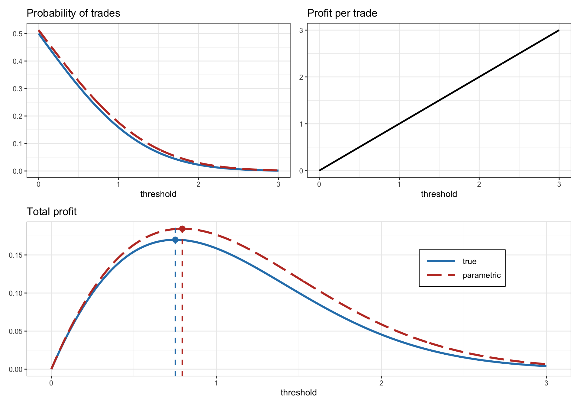
Figure 15.15: Calculation of optimum threshold in pairs trading via a parametric approach.
Nonparametric Data-Driven Approach
An alternative to the parametric approach (based on a probably inaccurate model) is a data-driven approach that does not rely on any model assumption. The idea is to simply use the available data to empirically count the number of tradable events for each possible threshold. Given \(T\) observations of the \(z\)-score, \(z^\textm{score}_t\) for \(t=1,\dots,T\), and \(J\) discretized threshold values, \(s_{01},\dots,s_{0J}\), we can compute the empirical trading frequency for each threshold \(s_{0j}\) (in one direction) as \[ \bar{f}_{j} =\frac{1}{T}\sum_{t=1}^{T}1{\{z^\textm{score}_t>s_{0j}\}}, \]
where \(1\{\cdot\}\) is the indicator function that equals 1 if the argument is true and zero otherwise.
Unfortunately, the empirical values \(\bar{f}_{j}\) can be very noisy, which can affect the assessment of the total profit. One way to reduce the noise in the values \(\bar{\bm{f}} = (\bar{f}_{1},\dots,\bar{f}_{J})\) is by taking advantage of the fact that the trading frequency should be a smooth function of the threshold. We can obtain a smoothed version by solving the least squares problem \[ \underset{\bm{f}}{\textm{minimize}} \quad \sum_{j=1}^{J}(f_{j} - \bar{f}_{j})^{2}+\lambda\sum_{j=1}^{J-1}(f_{j}-f_{j+1})^{2}, \] where the first term measures the difference between the noisy and smoothed values, and the second term enforces smoothness controlled by the hyper-parameter \(\lambda\). This problem can be rewritten with a compact notation as \[ \underset{\bm{f}}{\textm{minimize}} \quad \|\bm{f} - \bar{\bm{f}}\|_{2}^{2} + \lambda \|\bm{D}\bm{f}\|_{2}^{2}, \] where \(\bm{D}\) is a difference matrix defined as \[ \bm{D} = \begin{bmatrix} 1 & -1\\ & 1 & -1\\ & & \ddots & \ddots\\ & & & 1 & -1 \end{bmatrix} \in \R^{(J-1) \times J}. \] Since this problem is a least squares, we can write down the solution in closed form as \[ \bm{f}^{\star} = \left(\bm{I} + \lambda\bm{D}^\T\bm{D}\right)^{-1}\bar{\bm{f}}. \]
Finally, the optimal threshold can be obtained by maximizing the smoothed total profit: \[ s_{0}^{\star} = \underset{s_{0j}\in\{s_{01},s_{02},\dots,s_{0J}\}}{\textm{arg}\;\textm{max}} \, s_{0j} \times f_{j}. \] Figure 15.16 illustrates the nonparametric evaluation of the profit vs. the threshold for a synthetic Gaussian spread (both the original noisy version and the improved smoothed version).
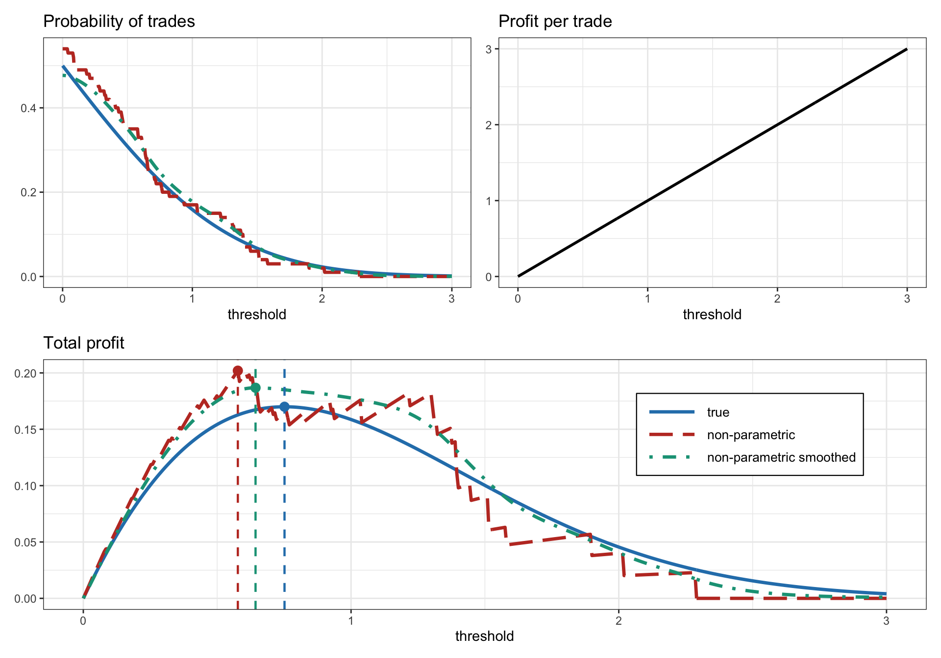
Figure 15.16: Calculation of optimum threshold in pairs trading via a nonparametric approach.
15.5.3 Numerical Experiments
We now execute pairs trading with market data examples during 2013–2022. The first two years are used to estimate the hedge factor \(\gamma\), which is critical to form the spread. Then the spread is traded over the remaining out-of-sample period. The \(z\)-score is computed on a rolling-window basis (as in Bollinger Bands) to make sure it adapts to the market changes over time and stays mean reverting. To trade the spread, the thresholded strategy is employed (the linear strategy can also be used with very similar results). For simplicity, the threshold is simply chosen as \(s_0=1\); of course it could be optimized but care has to be taken to avoid look-ahead bias and overfitting (see Chapter 8 for the dangers of backtesting and overfitting of hyper-parameters).
Market Data: EWA and EWC
We start with the two ETFs EWA and EWC, which track the performance of the Australian and Canadian economies, respectively. As previously checked in Section 15.4, the majority of the tests indicate that cointegration is present during most of the period, although in occasions it may be lost. The \(z\)-score is computed on a rolling-window basis with a lookback period of six months.
Figure 15.17 shows the spread (with hedge ratio \(\gamma\) estimated via least squares during the first two years), the \(z\)-score, the trading signal, and the cumulative return. We can observe that the spread does not show a strong persistent cointegration relationship over the whole period; in practice, the hedge ratio should be adapted over time. The \(z\)-score is able to produce a more constant mean-reverting version due to the rolling window adaptation. In any case, any practical implementation of pairs trading would recompute the hedge ratio over time, as assumed in the rest of the experiments via a rolling least squares.
Figure 15.18 shows the results when the hedge ratio \(\gamma\) is computed on a rolling-window basis with a lookback period of two years. We can appreciate that the spread has been improved compared to the previous fixed least squares and looks more mean-reverting. Still, the \(z\)-score is able to further improve it and produce a much better mean reverting version. The cumulative return shows the improvement thanks to the rolling least squares approach; nevertheless, it is much better to use the Kalman filter as explored in Section 15.6.
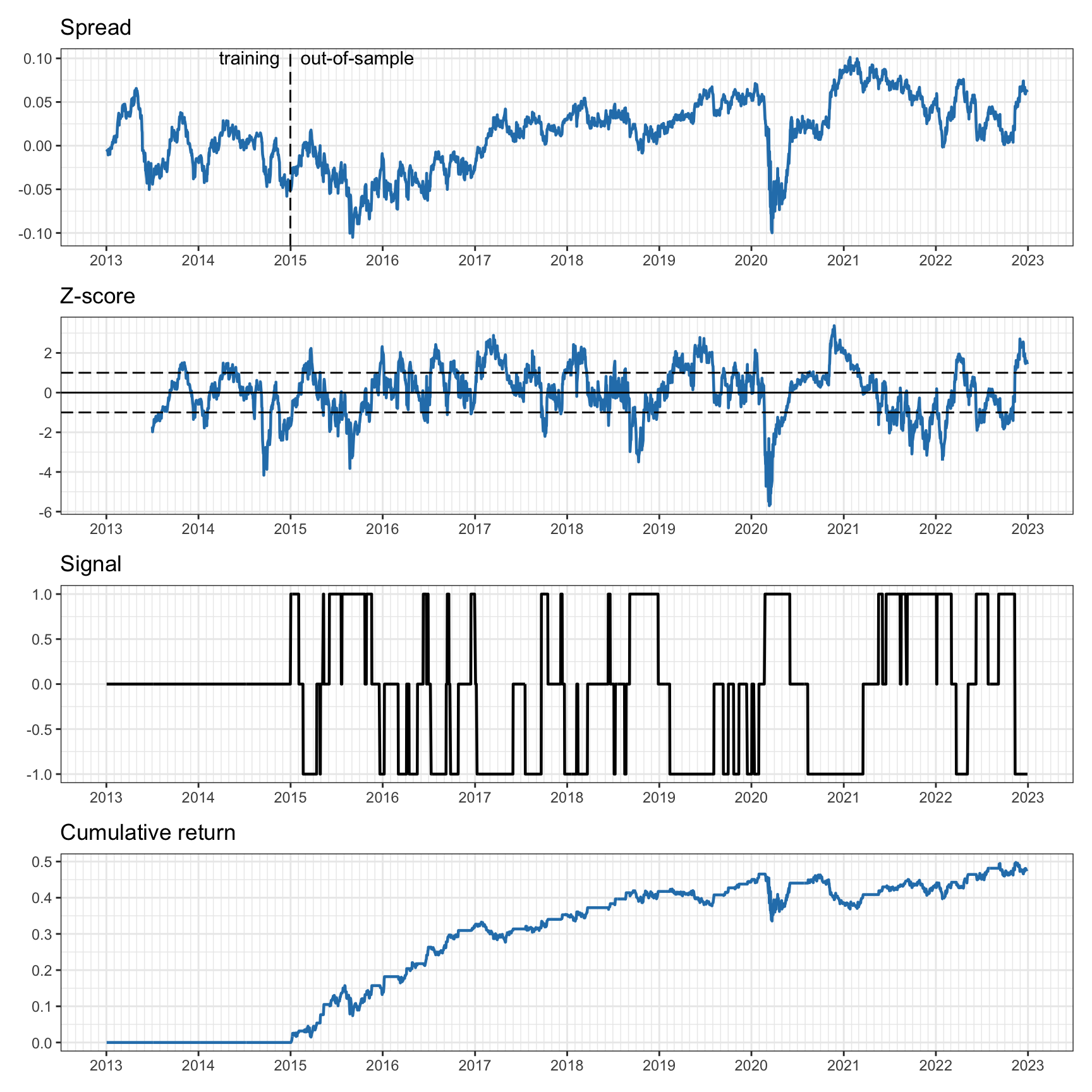
Figure 15.17: Pairs trading on EWA–EWC with six-month rolling \(z\)-score and two-year fixed least squares.
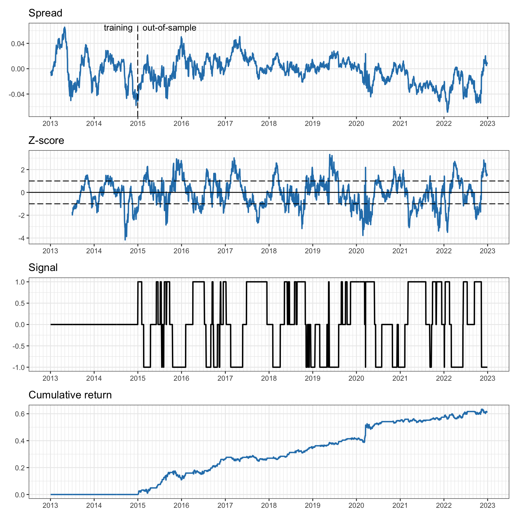
Figure 15.18: Pairs trading on EWA–EWC with six-month rolling \(z\)-score and two-year rolling least squares.
Market Data: KO and PEP
We continue with an attempt to execute pairs trading on the stocks Coca-Cola (KO) and Pepsi (PEP), which do not seem to be cointegrated according to the previous experiments in Section 15.4. To be realistic, the hedge ratio \(\gamma\) is estimated via a rolling least squares with a lookback period of two years (this may help in adapting to the changing cointegration relationship). The \(z\)-score is computed on a rolling-window basis with a lookback period of six months (as well as one month for a faster adaptation).
Figure 15.19 shows the spread, the \(z\)-score, the trading signal, and the cumulative return. We can observe that the spread loses the mean reversion property despite the rolling nature of the hedge ratio calculation. The \(z\)-score is able to produce a more constant mean-reverting version, but still one can observe jumps indicating loss of cointegration. The cumulative return indicates that trading is not very successful.
Figure 15.20 shows the results when the \(z\)-score is calculated with a faster adaptability using a lookback period of one month (as opposed to the previous six months). The \(z\)-score looks much better, with a strong mean reversion. This translates into higher-frequency trading (compare the frequency in the signals), but still the cumulative return does not seem to indicate good profitability.
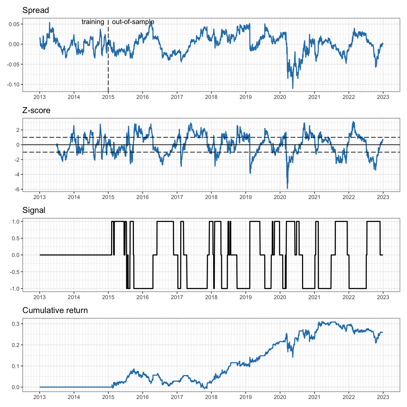
Figure 15.19: Pairs trading on KO–PEP with six-month rolling \(z\)-score and two-year rolling least squares.
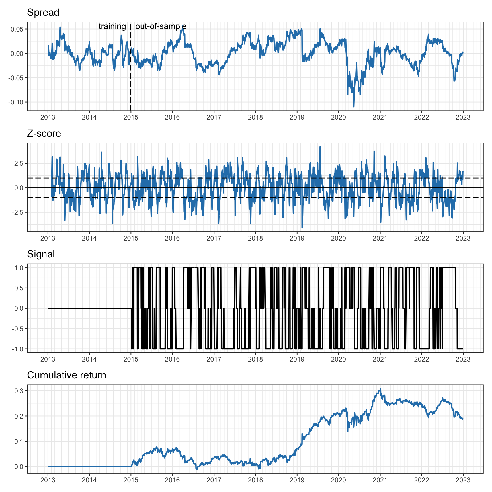
Figure 15.20: Pairs trading on KO–PEP with one-month rolling \(z\)-score and two-year rolling least squares.