6.5 Risk-Based Portfolios
We continue our exploration of portfolios with several risk-based portfolios that are solely based on risk considerations, characterized by the covariance matrix \(\bSigma\) (Ardia et al., 2017), while totally ignoring the return forecast \(\bmu\), due to the extremely noisy estimation of \(\bmu\) in practice (Chopra and Ziemba, 1993).
6.5.1 Global Minimum Variance Portfolio (GMVP)
In Section 6.3, we saw that the portfolio volatility \(\sqrt{\w^\T\bSigma\w}\) or, similarly, the variance \(\w^\T\bSigma\w\), can be used as proxies for portfolio risk. The global minimum variance portfolio (GMVP) is formulated as \[\begin{equation} \begin{array}{ll} \underset{\w}{\textm{minimize}} & \w^\T\bSigma\w\\ \textm{subject to} & \bm{1}^\T\w=1, \quad \w\ge\bm{0}. \end{array} \tag{6.14} \end{equation}\] This problem is a convex quadratic program (QP) that can be easily solved with a QP solver.
If we ignore the no-shorting constraint \(\w\ge\bm{0}\), then the problem admits the simple closed-form solution \[\begin{equation} \w = \frac{1}{\bm{1}^\T\bSigma^{-1}\bm{1}} \bSigma^{-1}\bm{1}. \tag{6.15} \end{equation}\]
This portfolio is widely used in academic papers for simplicity of evaluation, as well as for comparison purposes when evaluating different estimators of the covariance matrix \(\bSigma\) (while ignoring the effect of the estimation of \(\bmu\)).
6.5.2 Inverse Volatility Portfolio (IVolP)
The aim of the inverse volatility portfolio (IVolP) is to control the portfolio risk in a simple way. It is defined as \[\begin{equation} \w = \frac{\bm{\sigma}^{-1}}{\bm{1}^\T\bm{\sigma}^{-1}}, \tag{6.16} \end{equation}\] where \(\bm{\sigma}^2 = \textm{diag}\left(\bSigma\right)\) denotes the assets’ variances and \(\bm{\sigma}\) are the assets’ volatilities.
This portfolio allocates smaller weights to high-volatility assets and larger weights to low-volatility assets. It is also called equal volatility portfolio because the weighted constituent assets have equal volatility: \[ \textm{Std}(w_i r_i) = w_i \sigma_i \propto 1/N. \]
It is worth comparing the IVolP with the GMVP in (6.15) when the covariance matrix is assumed diagonal; in this case, the GVMP simplifies to \[ \w = \frac{\bm{\sigma}^{-2}}{\bm{1}^\T\bm{\sigma}^{-2}}, \] which, similary to (6.16), allocates smaller weights to high-volatility assets and vice versa.
6.5.3 Risk Parity Portfolio (RPP)
The risk parity portfolio (RPP), also termed equal risk portfolio (ERP), aims at equalizing the risk contribution from the invested assets to the global portfolio risk (Qian, 2005, 2016; Roncalli, 2013b). This portfolio design is extensively treated in Chapter 11 and here we provide a very concise summary.
The IVolP in (6.16) attempts to control the risk of each of the assets in a simple way, but it totally ignores the assets’ correlations, that is, it implicitly assumes that the covariance matrix \(\bSigma\) is diagonal. The RPP can be understood as a more sound formulation of the IVolP by properly taking the assets’ correlations into account.
The RPP attemps to equalize the risk contributions from the assets, reminiscent of the way the \(1/N\) portfolio equalizes the capital allocated to the assets, as shown in Figure 6.14.
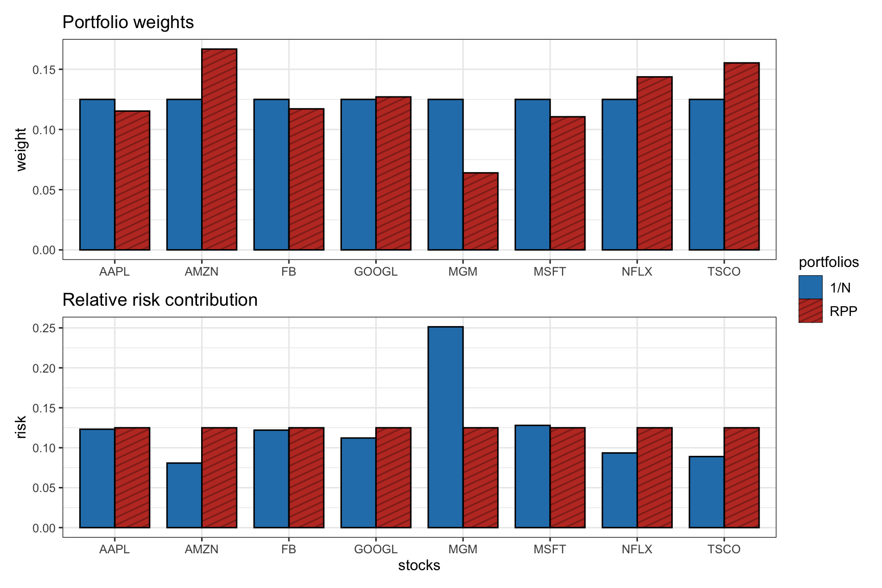
Figure 6.14: From dollar diversification (\(1/N\) portfolio) to risk diversification (RPP).
6.5.4 Most Diversified Portfolio (MDivP)
If markets are risk-efficient, it can be argued that assets will produce returns in proportion to their risk (Choueifaty and Coignard, 2008). This suggests that one might use a proxy for the assets’ risk, such as the volatilities, \(\bm{\sigma}\), in lieu of the forecast \(\bmu\).
Specifically, the diversification ratio (DR) is defined similarly to the Sharpe ratio (Section 6.3) but using \(\bm{\sigma}\) in lieu of \(\bmu\): \[\textm{DR} = \frac{\w^\T\bm{\sigma}}{\sqrt{\w^\T\bSigma\w}}.\] For long-only portfolios, it can be shown that \(\textm{DR}\ge1\) (for a single stock, it reduces to \(\textm{DR}=1\)).
The most diversified portfolio (MDivP) is formulated as the maximization of the DR (akin to the maximization of the Sharpe ratio considered in Section 7.2 from Chapter 7): \[\begin{equation} \begin{array}{ll} \underset{\w}{\textm{minimize}} & \dfrac{\w^\T\bm{\sigma}}{\sqrt{\w^\T\bSigma\w}}\\ \textm{subject to} & \bm{1}^\T\w=1, \quad \w\ge\bm{0}. \end{array} \tag{6.17} \end{equation}\]
6.5.5 Maximum Decorrelation Portfolio (MDecP)
The maximum decorrelation portfolio (MDecP) is defined similarly to the GMVP but using the correlation matrix \(\bm{C}\) in lieu of the covariance matrix \(\bSigma\) (Christoffersen et al., 2012): \[\begin{equation} \begin{array}{ll} \underset{\w}{\textm{minimize}} & \w^\T\bm{C}\w\\ \textm{subject to} & \bm{1}^\T\w=1, \quad \w\ge\bm{0}. \end{array} \tag{6.18} \end{equation}\] The correlation matrix \(\bm{C}\) can be interpreted as the covariance matrix of the normalized assets such that they have unit volatility, that is, \[\bm{C} = \textm{Diag}\left(\bSigma\right)^{-1/2} \bSigma \textm{Diag}\left(\bSigma\right)^{-1/2},\] where \(\textm{Diag}(\cdot)\) keeps the diagonal elements of the matrix argument and sets the off-diagonal elements to zero.
The MDecP is not only related to the GMVP but also to the MDivP: when the MDecP weights are divided by their respective assets’ volatilities and renormalized so that they sum to 1, the MDivP weights are obtained.
6.5.6 Numerical Experiments
We now compare the following risk-based portfolios: GMVP, IVolP, RPP, MDivP, and MDecP. We consider eight stocks from the S&P 500 during the period 2019–2020, under the same setting as the experiments in Section 6.4.5.
Figure 6.15 shows the normalized dollar allocation of the risk-based portfolios, whereas Figure 6.16 shows the out-of-sample backtest results in terms of cumulative P&L and drawdown. Since all these portfolios are precisely obtained by somehow minizing the risk, the resulting drawdowns are small (compare with the drawdowns of the heuristic portfolios in Figure 6.13).
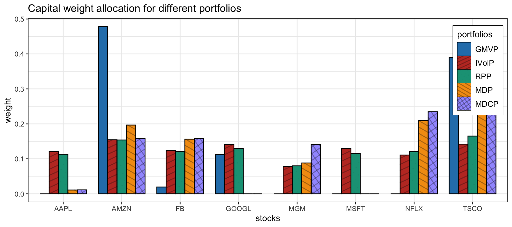
Figure 6.15: Portfolio allocation of risk-based portfolios.
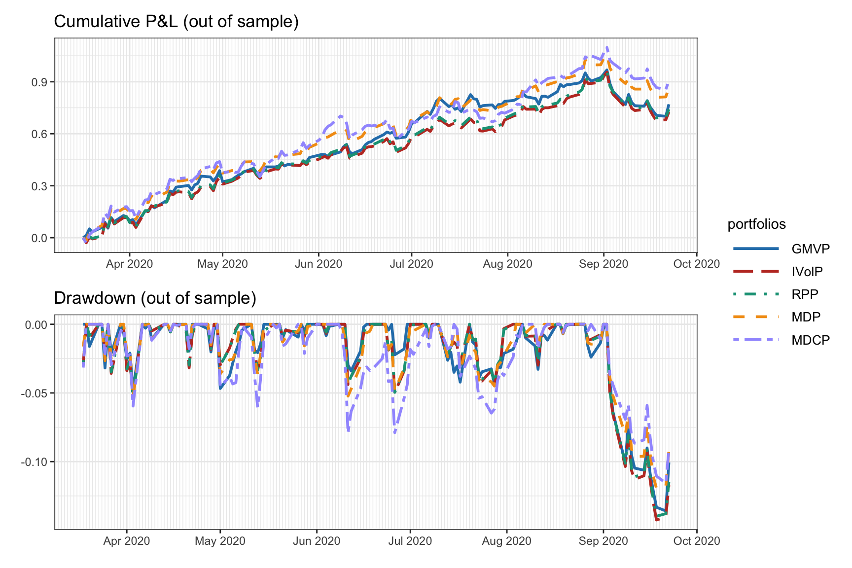
Figure 6.16: Backtest cumulative P&L and drawdown of risk-based portfolios.