5.2 Learning Graphs
In some applications, the graph structure can be readily obtained, such as in a social network where the nodes are the users and the connectivity can be measured by friendship relationships. In many other practical scenarios, however, the underlying graph structure is not directly observable and has to be inferred from the data, such as in a gene graph, brain activity graph, or a financial graph.
Numerous methods for learning graphs have been proposed in recent decades, ranging from heuristic techniques based on the physical interpretation of graphs to more statistically sound approaches that build upon well-established results from estimation theory.
The starting point in a graph learning method from data is the data matrix, \[\begin{equation} \bm{X}=[\bm{x}_1,\bm{x}_2,\dots,\bm{x}_p]\in\R^{n\times p}, \tag{5.2} \end{equation}\] where each column contains the signal of one variable or node, \(p\) is the number of variables or nodes, and \(n\) is the length of the signal or number of observations. In the context of financial time series, the number of observations is often denoted by \(T\) instead of \(n\), and the number of nodes or assets is often denoted by \(N\) instead of \(p\). Each row of matrix \(\bm{X}\) represents one observation of the signal on the graph, called the graph signal.
The goal in graph learning is to transition from the data matrix \(\bm{X}\) to the graph description \(\mathcal{G}=(\mathcal{V},\mathcal{E},\bm{W})\) as illustrated in Figure 5.4. A simple example of graph learning from data is depicted in Figure 5.5, where the nodes are points in \(\R^2\) sampled from the “two-moon” dataset, and the resulting graph clearly comprises two components corresponding to the two moons.
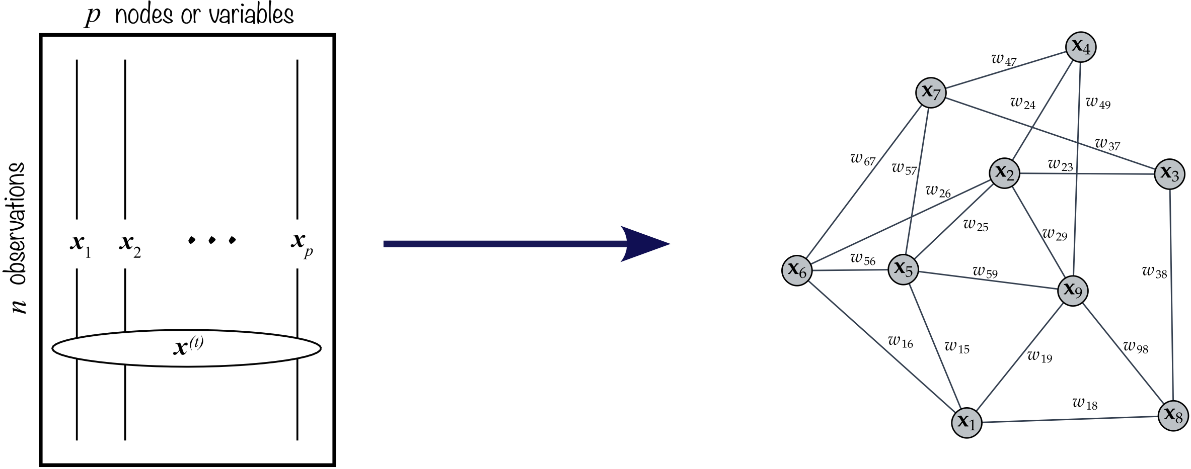
Figure 5.4: Learning a graph from data.
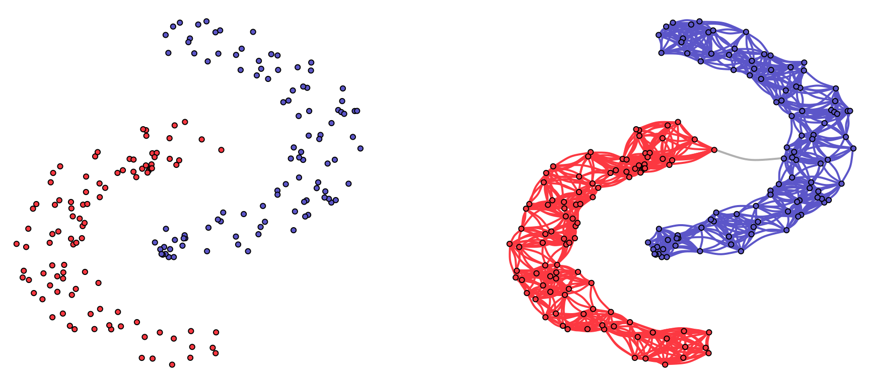
Figure 5.5: Illustration of graph learning for a toy example.
The field of graph learning has experienced significant growth in recent years, with numerous studies introducing enhanced graph estimation techniques in terms of both quality and computational efficiency.
In what appears to be a pioneering effort, the seminal paper of Mantegna (1999) was the first to implement data-driven graphs in financial markets, employing a straightforward correlation graph.
For a comprehensive understanding of graph theory, the standard textbooks Lauritzen (1996) and Kolaczyk (2009) provide excellent coverage.
For introductory and overview articles on graph learning, refer to Mateos et al. (2019) and Dong et al. (2019).
Basic graph learning algorithms are found in Lake and Tenenbaum (2010), Egilmez et al. (2017), and L. Zhao et al. (2019).
Structured graph learning: A general approach via spectral constraints is proposed in Kumar et al. (2019) and Kumar et al. (2020), graphs with sparsity are studied in Ying et al. (2020), and a convex formulation for bipartite graphs is developed in Cardoso et al. (2022a).
Graph learning with financial data: General guidelines for financial time series are considered in Cardoso and Palomar (2020), learning under heavy tails is explored in Cardoso et al. (2021), and the application of bipartite-structured graphs for clustering is considered in Cardoso et al. (2022a); an overview is given in Cardoso et al. (2022b).
A comprehensive overview of the literature on financial graphs in the past two decades can be found in Marti et al. (2021).
5.2.1 Learning Graphs from Similarity Measures
The simplest methods to infer a graph from data are based on computing each element of the adjacency matrix \(\bm{W}\) (either weighted or \(0\)–\(1\) connectivity) by measuring the connectivity strength between each pair of nodes one by one. To measure the strength, a wide variety of similarity functions or scoring functions can be used (Kolaczyk, 2009), leading to totally different graphs.
For illustration purposes, a few simple methods are listed next based on the data matrix \(\bm{X}\in\R^{n\times p}\) defined in (5.2), where the \(i\)th column \(\bm{x}_i\in\R^n\) corresponds to the signal at node \(i\):
Thresholded distance graph: Nodes \(i\) and \(j\) are connected (\(w_{ij}=1\)) if the corresponding signals satisfy \(\|\bm{x}_i - \bm{x}_j\|^2 \le \gamma\), where \(\gamma\) is a threshold; otherwise not connected (\(w_{ij}=0\)).
Gaussian graph: Set every pair of points \(i\neq j\) as connected with the Gaussian weights \[w_{ij} = \textm{exp}\left(-\frac{\|\bm{x}_i - \bm{x}_j\|^2}{2\sigma^2}\right),\] where \(\sigma^2\) controls the size of the neighborhood.
\(k\)-nearest neighbors (\(k\)-NN) graph: Nodes \(i\) and \(j\) are connected (\(w_{ij}=1\)) if \(\bm{x}_i\) is one of the \(k\) closest points to \(\bm{x}_j\) or vice versa; otherwise not connected (\(w_{ij}=0\)).
Feature correlation graph: Simply use pairwise feature correlation for \(i\neq j\): \[w_{ij} = \bm{x}_i^\T\bm{x}_j.\] It is worth noting that if the signals are normalized (i.e., \(\|\bm{x}_i\|^2=1\)), then the Euclidean distance used in the Gaussian weights is directly related to the correlation: \(\|\bm{x}_i - \bm{x}_j\|^2 = 2\times (1 - \bm{x}_i^\T\bm{x}_j).\)
However, because the connectivity of each pair is measured independently of the others, these heuristic methods do not provide holistic measures and may not perform well in practice, especially for time series data. In principle, it is better to measure the connectivity of all pairs all at once in a joint manner, as explored in the next sections.
5.2.2 Learning Graphs from Smooth Signals
We will now derive a family of graph learning methods based on the measure of smoothness or variance of a graph signal defined in (5.1). To recall, given a \(p\)-dimensional graph signal \(\bm{x}\) (defined on a graph with \(p\) nodes), a natural measure of its variance on the graph is \(\bm{x}^\T\bm{L}\bm{x} = \frac{1}{2}\sum_{i,j}W_{ij}(x_i - x_j)^2.\)
Suppose now we have \(n\) observations of graph signals contained in the data matrix \(\bm{X}\in\R^{n\times p}\) defined in (5.2), where the \(i\)th column \(\bm{x}_i\in\R^n\) corresponds to the signal at node \(i\) and the \(t\)-th observation of the graph signal \(\bm{x}^{(t)}\in\R^p\) is contained along the \(t\)-th row.
The overall variance corresponding to the \(n\) observations contained in the data matrix \(\bm{X}\) can be written in terms of the Laplacian matrix \(\bm{L}\) as \[ \sum_{t=1}^n(\bm{x}^{(t)})^\T\bm{L}\bm{x}^{(t)} = \textm{Tr}\left(\bm{X}\bm{L}\bm{X}^\T\right) \] or, equivalently, in terms of the adjacency matrix \(\bm{W}\) as \[ \sum_{t=1}^n \frac{1}{2}\sum_{i,j}W_{ij}\left(x^{(t)}_i - x^{(t)}_j\right)^2 = \frac{1}{2}\sum_{i,j}W_{ij}\|\bm{x}_i - \bm{x}_j\|^2 = \frac{1}{2}\textm{Tr}(\bm{W}\bm{Z}), \] where the matrix \(\bm{Z}\) contains the squared Euclidean distances between signals: \(Z_{ij} \triangleq \|\bm{x}_i - \bm{x}_j\|^2\).
Now that we have expressed the variance of a collection of signals on a graph, we are ready to formulate the graph learning problem. The key observation is that if a signal has been generated by a graph, then it is expected to have a small variance as measured on that graph. This is a natural assumption because if two nodes are strongly connected, then the signals on these two nodes should be similar; alternatively, if two nodes are not connected, then the corresponding signals can be totally different.
Based on this assumption on the signal smoothness measured on the generating graph, suppose we collect some graph signals in the data matrix \(\bm{X}\) with the hypothesis that they could have been generated either by graph \(\mathcal{G}_1\) or \(\mathcal{G}_2\), with corresponding Laplacian matrices \(\bm{L}_1\) and \(\bm{L}_2\), respectively. Then, to determine which graph has generated the data, we simply have to compute the signal variance on each of the two graphs, \(\textm{Tr}\left(\bm{X}\bm{L}_1\bm{X}^\T\right)\) and \(\textm{Tr}\left(\bm{X}\bm{L}_2\bm{X}^\T\right)\), and choose the one with the smaller variance.
We can now take the previous problem of choosing a graph among a set of possible alternatives to the next level. Suppose again we collect some graph signals in the data matrix \(\bm{X}\) and want to determine the graph \(\mathcal{G}\) that best fits the data in the sense of producing a minimum signal variance. That is, we want to determine the graph (either in terms of \(\bm{L}\) or \(\bm{W}\)) that gives the minimum signal variance on that graph. In addition, for practical purposes, we may want to include a regularization term on the estimated graph to control some other graph properties, such as sparsity, energy, or volume.
Thus, the simplest problem formulation in terms of the Laplacian matrix \(\bm{L}\) is \[\begin{equation} \begin{array}{ll} \underset{\bm{L}\succeq\bm{0}}{\textm{minimize}} & \textm{Tr}\left(\bm{X}\bm{L}\bm{X}^\T\right) + \gamma h_L(\bm{L})\\ \textm{subject to} & \bm{L}\bm{1}=\bm{0}, \quad L_{ij} = L_{ji} \le 0, \quad \forall i\neq j, \end{array} \tag{5.3} \end{equation}\] where \(\gamma\) is a hyper-parameter to control the regularization level and \(h_L(\bm{L})\) is a regularization function, e.g., \(\|\bm{L}\|_1\), \(\|\bm{L}\|_\textm{F}^2\), or \(\textm{volume}(\bm{L})\). Observe that this formulation incorporates as constraints the structural properties that the Laplacian matrix is supposed to satisfy (see Section 5.1.2).
Similarly, the simplest problem formulation in terms of the adjacency matrix \(\bm{W}\) is \[\begin{equation} \begin{array}{ll} \underset{\bm{W}}{\textm{minimize}} & \frac{1}{2}\textm{Tr}(\bm{W}\bm{Z}) + \gamma h_W(\bm{W})\\ \textm{subject to} & \textm{diag}(\bm{W})=\bm{0}, \quad \bm{W}=\bm{W}^\T \ge \bm{0}, \end{array} \tag{5.4} \end{equation}\] where \(h_W(\bm{W})\) is a regularization function for the adjacency matrix. As before, this formulation incorporates as constraints the structural properties that the adjacency matrix is supposed to satisfy (see Section 5.1.2).
It is worth noting that these formulations are convex provided that the regularization terms are convex functions. It may seem that the formulation in terms of the Laplacian matrix in (5.3) has a higher complexity than (5.4) due to the positive semidefinite matrix constraint \(\bm{L}\succeq\bm{0}.\) However, this is not the case because \(\bm{L}\succeq\bm{0}\) is implied by the other two sets of linear constraints, \(\bm{L}\bm{1}=\bm{0}\) and \(L_{ij} = L_{ji} \le 0\) for \(i\neq j\) (Ying et al., 2020).
Controlling the Degrees of the Nodes
Controlling the degrees of the nodes in a graph is important to avoid the problem of unbalanced graphs or even isolated nodes in the graph. Recall from Section 5.1.2 that the degrees of the nodes in a graph are given by \(\bm{d}=\bm{W}\bm{1}\).
Some examples of graph learning with degree control include:
Sparse graphs with fixed degrees: The formulation in (5.4) was adopted in Nie et al. (2016) with the regularization term \(\|\bm{W}\|_\textm{F}^2\) to control the sparsity of the graph and the constraint \(\bm{W}\bm{1} = \bm{1}\) to control the degrees of the nodes.
Sparse graphs with regularized degrees: An alternative to fixing the degrees as \(\bm{W}\bm{1} = \bm{1}\) is to include a regularization term in the objective such as \(-\bm{1}^\T\textm{log}(\bm{W}\bm{1})\) (Kalofolias, 2016).
Robust graphs against noisy data: Since observations are often noisy, a robust version of the smoothness term \(\textm{Tr}\left(\bm{X}\bm{L}\bm{X}^\T\right)\) in (5.3) was proposed in Dong et al. (2015) by combining the term \(\textm{Tr}\left(\bm{Y}\bm{L}\bm{Y}^\T\right)\) with \(\|\bm{X} - \bm{Y}\|_\textm{F}^2\), where \(\bm{Y}\) attempts to remove the noise in \(\bm{X}\).
5.2.3 Learning Graphs from Graphical Model Networks
In the previous sections, the data matrix \(\bm{X}\) was assumed to contain the graph data without any statistical modeling. Alternatively, the graph learning process can be formulated in a more sound way as a statistical inference problem. We will now assume that the graph signals contained along the rows of \(\bm{X}\), denoted by \(\bm{x}^{(t)},\; t=1,\dots,T,\) where \(T\) is the number of observations, follow some multivariate distribution such as the Gaussian distribution, \[\bm{x}^{(t)} \sim \mathcal{N}(\bmu, \bSigma),\] where \(\bmu\) is the mean vector and \(\bSigma\) the covariance matrix of the observations. Later, in Section 5.4, more realistic heavy-tailed distributions will be considered.
Recall that, in practice, the covariance matrix \(\bSigma\) is typically estimated via the sample covariance matrix \[ \bm{S} = \frac{1}{T}\sum_{t=1}^T (\bm{x}^{(t)} - \bmu)(\bm{x}^{(t)} - \bmu)^\T = \frac{1}{T} \big(\bm{X} - \bm{\bar{X}}\big)^\T\big(\bm{X} - \bm{\bar{X}}\big), \] where the matrix \(\bm{\bar{X}}\) contains \(\bmu\) along each row (see Chapter 3 for more details on the estimation of covariance matrices).
The topic of estimation of graphical models goes back at least to the 1970s, when the inverse sample covariance matrix \(\bm{S}^{-1}\) was proposed to determine a graph (Dempster, 1972). Some paradigmatic examples of network graph construction include the following:
- Correlation networks: The correlation between two random variables characterizes the similarity between them (at least in a linear sense). Therefore, it can be used as a way to measure how similar two nodes are and, hence, as a way to characterize a graph (Kolaczyk, 2009; Lauritzen, 1996). Nevertheless, a big drawback of using correlations is that two nodes may have a high correlation through a dependency on other nodes. For example, in the context of financial data, it is well known that all the stocks are significantly driven by a few factors. As a consequence, they all exhibit a high correlation that does not really characterize the similarity between stocks once the factors are accounted for.
Partial correlation networks: The correlation measures the direct dependency between two nodes but ignores the other nodes. A more refined version is to measure the dependency but conditioned on the other nodes, that is, factoring out the effect of other nodes. For example, height and vocabulary of children are not independent, but they are conditionally independent conditioned on age.
Interestingly, all the information of partial correlation and dependency conditioned on the rest of the graph is contained in the so-called precision matrix defined as \(\bm{\Theta} = \bSigma^{-1}\), that is, the inverse covariance matrix. To be precise, the correlation between nodes \(i\) and \(j\), conditioned on the rest of the nodes of the network, is equal to \(-\Theta_{ij}/\sqrt{\Theta_{ii}\Theta_{jj}}\) (Kolaczyk, 2009; Lauritzen, 1996). As a consequence, two nodes \(i\) and \(j\) are conditionally independent if and only if \(\Theta_{ij}=0\).
A graph defined by the precision matrix is called a partial correlation network or conditional dependence graph. In such a graph, nonzero off-diagonal entries of the precision matrix \(\bm{\Theta}\) correspond to the edges of the graph.
- Graphical LASSO (GLASSO): This method tries to estimate a sparse precision matrix (O. Banerjee et al., 2008; Friedman et al., 2008). Assuming a multivariate Gaussian distribution function for the data, the regularized maximum likelihood estimation of the precision matrix \(\bm{\Theta} = \bSigma^{-1}\) can be formulated (refer to Section 3.4 in Chapter 3) as \[\begin{equation} \begin{array}{ll} \underset{\bm{\Theta}\succ\bm{0}}{\textm{maximize}} & \textm{log det}(\bm{\Theta}) - \textm{Tr}(\bm{\Theta}\bm{S}) - \rho\|\bm{\Theta}\|_{1,\textm{off}}, \end{array} \tag{5.5} \end{equation}\] where \(\|\cdot\|_{1,\textm{off}}\) denotes the elementwise \(\ell_1\)-norm of the off-diagonal elements and the hyper-parameter \(\rho\) controls the level of sparsity of the precision matrix. The regularization term \(\|\bm{\Theta}\|_{1,\textm{off}}\) enforces learning a sparse precision matrix.
- Laplacian-structured GLASSO: The precision matrix plays a role in graphs similar to the Laplacian matrix in the context of Gaussian Markov random fields (GMRFs) (Rue and Held, 2005). Under that setting, the GLASSO formulation in (5.5) can be reformulated to include the Laplacian constraints (Egilmez et al., 2017; Lake and Tenenbaum, 2010; L. Zhao et al., 2019) as22 \[\begin{equation} \begin{array}{ll} \underset{\bm{L}\succeq\bm{0}}{\textm{maximize}} & \textm{log gdet}(\bm{L}) - \textm{Tr}(\bm{L}\bm{S}) - \rho\|\bm{L}\|_{1,\textm{off}}\\ \textm{subject to} & \bm{L}\bm{1}=\bm{0}, \quad L_{ij} = L_{ji} \le 0, \quad \forall i\neq j, \end{array} \tag{5.6} \end{equation}\] where \(\textm{gdet}\) denotes the generalized determinant defined as the product of nonzero eigenvalues (this is necessary because, differently from \(\bm{\Theta}\succ\bm{0}\) in (5.5), the Laplacian \(\bm{L}\) is singular due to the constraint \(\bm{L}\bm{1}=\bm{0}\)).
Sparse GMRF graphs: The Laplacian-structured GLASSO in (5.6) is an improvement over the vanilla GLASSO in (5.5). However, rather surprisingly, the \(\ell_1\)-norm regularization term \(\|\bm{L}\|_{1,\textm{off}}\) produces dense graphs instead of sparse ones (Ying et al., 2020). Thus, a more appropriate formulation for sparse GMRF graphs is (Kumar et al., 2020; Ying et al., 2020) 23 \[\begin{equation} \begin{array}{ll} \underset{\bm{L}\succeq\bm{0}}{\textm{maximize}} & \textm{log gdet}(\bm{L}) - \textm{Tr}(\bm{L}\bm{S}) - \rho\|\bm{L}\|_{0,\textm{off}}\\ \textm{subject to} & \bm{L}\bm{1}=\bm{0}, \quad L_{ij} = L_{ji} \le 0, \quad \forall i\neq j. \end{array} \tag{5.7} \end{equation}\]
The sparsity regularization term \(\|\bm{L}\|_{0,\textm{off}}\) is a difficult function to deal with, being nonconvex, nondifferentiable, and noncontinuous. In practice, it can be approximated with a smooth concave function \(\sum_{ij}\phi(L_{ij}),\) with \(\phi\) concave, such as \(\phi(x) = \textm{log}(\epsilon + |x|),\) where the parameter \(\epsilon\) is a small positive number, and then this concave function can be successively approximated by a convex weighted \(\ell_1\)-norm (via the majorization–minimization method (Y. Sun et al., 2017), see Section B.7 in Appendix B for details), leading to the so-called reweighted \(\ell_1\)-norm regularization method (Candès et al., 2008), which has been successfully employed for sparse graph learning (Cardoso et al., 2022b; Kumar et al., 2020; Ying et al., 2020).
5.2.4 Numerical Experiments
For the empirical analysis, we use three years’ worth of stock price data (2016–2019) from the following three sectors of the S&P 500 index: Industrials, Consumer Staples, and Energy. The data matrix \(\bm{X}\in\R^{T\times N}\) is created with the log-returns of the \(N\) assets.
Since different assets can show widely different volatilities, it is convenient to normalize them so that each has volatility one (normalizing the data is equivalent to using the correlation matrix in lieu of the covariance matrix). In fact, in machine learning it is almost always the case that data is normalized prior to the application of any method; this is to avoid problems arising from different dynamic ranges in the data or even different units of measurement.
It is worth pointing out that, as previously mentioned in Section 5.2.3, financial assets typically present a high correlation due to the market factor or other few factors (see Chapter 3). One may be tempted to remove the effect of these factors and then learn the graph based on the residual idiosynchratic component. However, the precision matrix (and the Laplacian matrix) have an interpretation of partial correlation, which means that the effect of common factors affecting other nodes is already removed.
Among all the methods explored in this section, the most appropriate for time series are the GMRF-based methods enforcing graph sparsity either via the \(\ell_1\)-norm (the Laplacian-structured GLASSO formulation in (5.6)) or via the \(\ell_0\) penalty term (the sparse GMRF graph formulation (5.7)), which in practice is solved with a reweighted \(\ell_1\)-norm iterative method. Figure 5.6 shows the graphs obtained with these two methods, demonstrating the superior performance of the reweighted \(\ell_1\)-norm iterative method.
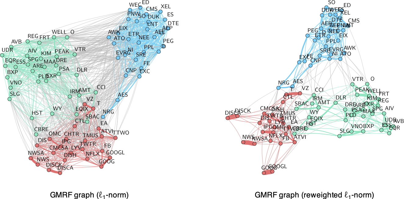
Figure 5.6: Effect of sparsity regularization term on financial graphs.
References
The R package
spectralGraphTopologycontains the functionlearn_laplacian_gle_admm()to solve problem (5.6) (Cardoso and Palomar, 2022). ↩︎The R package
sparseGraphcontains the functionlearn_laplacian_pgd_connected()to solve problem (5.7). ↩︎