9.1 Introduction
Markowitz’s mean–variance portfolio (Markowitz, 1952) formulates the portfolio design as a trade-off between the expected return \(\w^\T\bmu\) and the risk measured by the variance \(\w^\T\bSigma\w\) (see Chapter 7 for details): \[ \begin{array}{ll} \underset{\w}{\textm{maximize}} & \w^\T\bmu - \frac{\lambda}{2}\w^\T\bSigma\w\\ \textm{subject to} & \w \in \mathcal{W}, \end{array} \] where \(\lambda\) is a hyper-parameter that controls the investor’s risk aversion and \(\mathcal{W}\) denotes an arbitrary constraint set, such as \(\mathcal{W} = \{\w \mid \bm{1}^\T\w=1, \w\ge\bm{0} \}\).
Nevertheless, decades of empirical studies have clearly demonstrated that financial data do not follow a Gaussian distribution (see Chapter 2 for stylized facts of financial data). This implies that it would be reasonable to also incorporate higher-order moments (or higher-order statistics), in addition to the first two moments (i.e., mean and variance), in the portfolio formulation. We will consider here the first four moments as an improvement over the first two moments. The third and fourth moments are called skewness and kurtosis, respectively. In terms of portfolio optimization, in the same way that a higher expected return and lower variance are desired, we should seek a higher skewness and a lower kurtosis (i.e., higher odd moments and lower even moments) (Scott and Horvath, 1980).
Figure 9.1 shows the skewed \(t\) probability distribution function with different degrees of skewness (controlled by the parameter \(\gamma\), with \(\gamma=0\) for the symmetric case) and kurtosis (controlled by the parameter \(\nu\), with \(\nu\rightarrow\infty\) for the non-heavy-tailed case).
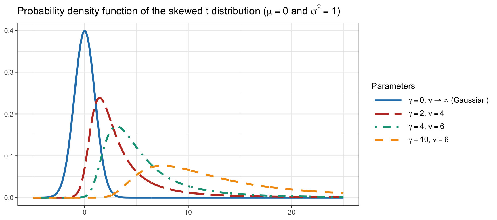
Figure 9.1: Illustration of skewness and kurtosis with the skewed \(t\) distribution.
The higher moments are definitely important and, for example, a skew-adjusted Sharpe ratio was proposed in Zakamouline and Koekebakker (2009): \[ \textm{skew-adjusted-SR} = \textm{SR} \times \sqrt{1 + \frac{\textm{skewness}}{3}\textm{SR}}. \]
Thus, the idea is to have a portfolio formulation where investors may accept lower expected return and/or higher volatility, compared to the mean–variance benchmark, in exchange for higher skewness and lower kurtosis.
9.1.1 High-Order Portfolios
As will be elaborated in the next section, the third and fourth moments of the portfolio are given by the expressions \(\w^\T\bm{\Phi}(\w\otimes\w)\) and \(\w^\T\bm{\Psi}(\w\otimes\w\otimes\w)\), respectively, where \(\bm{\Phi} \in \R^{N\times N^2}\) is the co-skewness matrix, and \(\bm{\Psi} = \in \R^{N\times N^3}\) is the co-kurtosis matrix.
Unfortunately, the incorporation of the third and fourth moments into the portfolio formulation brings two critical issues:
- Due to the dimensions of the co-skewness and co-kurtosis matrices, their computation, storage in memory, and algorithmic manipulation will be extremely challenging and severely limiting.
- The third moment is a nonconvex function of the portfolio \(\w\). This will make the high-order portfolio formulations complicated and the design of numerical algorithms more involved.
9.1.2 Historical Perspective
Portfolio formulations incorporating high-order moments go back to the 1960s (Jean, 1971; W. E. Young and Trent, 1969). However, the estimation of such high-order moments was an absolute impasse in those early days, the main problem being the dimensionality issue (recall that the co-skewness matrix is \(N\times N^2\) and the co-kurtosis matrix is \(N\times N^3\)), which means that the number of parameters quickly grows with the number of assets, with detrimental consequences in terms of the amount of data required for the estimation, the computational cost, and the storage needs. As a consequence, some authors have shown skepticism regarding the portfolio formulation based on high-order moments (Brandt et al., 2009):
extending the traditional approach beyond first and second moments, when the investor’s utility function is not quadratic, is practically impossible because it requires modeling [ …] the numerous higher-order cross-moments.
We had to wait for half a century to start finding publications proposing improved estimation methods, such as introducing structure and shrinkage in the high-order parameters (Boudt et al., 2014; Martellini and Ziemann, 2010) or assuming parametric multivariate distributions, to drastically reduce the number of parameters to estimate (Birgeand and Chavez-Bedoya, 2016; X. Wang et al., 2023). As empirically shown in Martellini and Ziemann (2010), unless improved estimators are employed, incorporating third and fourth moments in the portfolio design is detrimental in terms of out-of-sample performance.
In addition, apart from the estimation difficulties, the algorithmic part of the portfolio design has been extremely challenging. Since the high-order problem formulations are nonconvex, one approach is to use meta-heuristic optimization tools, such as genetic algorithms or differential evolution (Boudt et al., 2014), which attempt to find the global solution at the expense of a very high computational cost, but this becomes prohibitive when the problem dimension grows. Local optimization methods are a reasonable practical alternative by finding a locally optimal solution with acceptable computational cost.
A method based on difference-of-convex (DC) programming was proposed to solve high-order portfolio problems to a stationary point (Dinh and Niu, 2011), but convergence is slow and it is only applicable to low-dimensional problems. An improved method was proposed based on the difference of convex sums of squares (DC-SOS) decomposition techniques (Niu and Wang, 2019), but the complexity of computing the gradients of high-order moments grows rapidly with the problem dimension. The classical gradient descent method and backtracking line search also become inapplicable when the problem dimension grows large.
Faster methods were developed in Zhou and Palomar (2021) based on the successive convex approximation (SCA) framework (Scutari et al., 2014), which solves the original difficult problem by constructing and solving a sequence of convex approximated problems whose solutions converge to a stationary point of the original problem (see Appendix B for details on the SCA framework). The obtained algorithms converge much faster, although each iteration still requires a significant computational cost due to the computation of gradients and Hessians of high-order moments, allowing high-dimensional settings on the order of hundreds of assets, but not higher.
In Birgeand and Chavez-Bedoya (2016) and X. Wang et al. (2023), the computational cost of high-order moments was significantly reduced via a multivariate parametric model of the data, and in X. Wang et al. (2023) even faster numerical methods were developed that can be employed in very large dimensions with hundreds or thousands of assets.
Thus, practical high-order portfolios are now a reality after more than half a century of research by the scientific community.