8.1 A Typical Backtest
A backtest is a historical simulation of a strategy in some past period of time. We can see backtest results in academic publications, fund brochures, practitioner blogs, and so on.
Since strategies typically require the estimation of some parameters, such as the assets’ expected return vector \(\bmu\) or covariance matrix \(\bSigma\), the data is commonly split into an in-sample dataset, which acts as historical data that can be used to estimate parameters, and an out-of-sample dataset, which serves as “future” data that is used to assess the performance.
As an illustrative example, suppose we want to evaluate three portfolios: the \(1/N\) portfolio (see Section 6.4.3), the inverse volatility portfolio (IVolP) (see Section 6.5.2), and the global minimum variance portfolio (GMVP) (see Section 6.5.1). Figure 8.1 shows the cumulative P&L and drawdown of these portfolios. This gives an assessment of the behavior of the portfolios over time. In addition, Table 8.1 provides more concrete numerical values of different performance measures over the whole period.
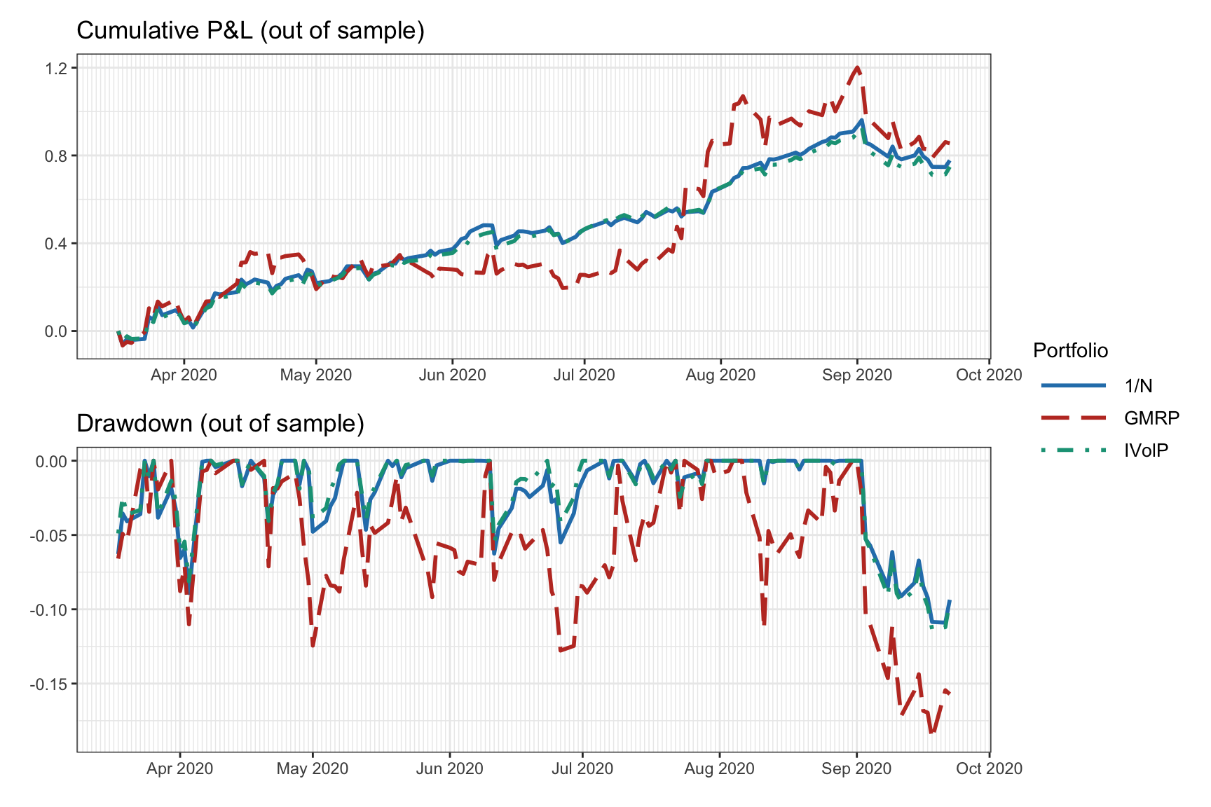
Figure 8.1: Example of a backtest result in the form of cumulative P&L and drawdown plots.
| Portfolio | Sharpe ratio | Annual return | Annual volatility | Sortino ratio | Max drawdown | CVaR (0.95) |
|---|---|---|---|---|---|---|
| 1/\(N\) | 3.23 | 117% | 36% | 5.40 | 11% | 5% |
| GMRP | 2.19 | 138% | 63% | 4.09 | 19% | 7% |
| IVolP | 3.35 | 113% | 34% | 5.61 | 11% | 4% |
Of course, more detailed results could be provided, such as a rolling Sharpe ratio plot over time (see Section 6.3.4) or a table with performance measures on a monthly basis instead of the overall annualized values. The reader is referred to Section 6.3 for a list of common performance measures.
The Global Investment Performance Standard (GIPS)40 is a set of standardized, industry-wide ethical principles that apply to the way investment performance is presented to potential and existing clients of asset managers, regulators, pension funds, financial advisers, and financial companies from around the globe. These standards guide investment firms on how to calculate and present their investment results to prospective clients. GIPS are standards, not laws. Firms do not have to be GIPS compliant; however, the standards provide discipline and claiming compliance with them demonstrates a firm-wide commitment to ethical best practices and that the firm employs strong internal control processes.
Nevertheless, the fact of the matter is that all these backtest results only provide very limited information on the real performance of the portfolios and, even worse, most likely the results are faulty and misleading. Indeed, this is clearly stated by notable authors, such as C. R. Harvey et al. (2016): “Most claimed research findings in financial economics are likely false,” and López de Prado (2018a), “Most backtests published in journals are flawed, as the result of selection bias on multiple tests.”
Sections 8.2 and 8.3 explore the many ways in which backtests are misleading and can provide wrong results. Then, Sections 8.4 and 8.5 go over details on how to execute backtests as safe as possible. A brief summary is then given in Section 8.6.