7.5 Drawbacks
Markowitz’s mean–variance portfolio, while great in theory, is dangerous in practice, so practitioners use it with caution. It has even been referred to as the “Markowitz optimization enigma” and sometimes the portfolio optimization is referred to as “error maximizer” (Michaud, 1989). There are multiple reasons for this, and academics and practitioners have proposed improvements and alternatives since Markowitz’s seminal paper (Markowitz, 1952). As stated in Michaud (1989):
… it remains one of the outstanding puzzles of modern finance that MV optimization has yet to meet with widespread acceptance by the investment community…
The extensions and improvements to the basic MVP are endless. To name a few: improved parameter estimation via shrinkage estimators or Black–Litterman-style approaches, robust portfolio optimization, alternative measures of risk, modeling of transaction costs, and multi-period portfolio optimization (see Kolm et al. (2014)). We next elaborate on some of these points.
7.5.1 Noisy Estimation of the Expected Returns
It has long been recognized that mean–variance efficient portfolios constructed using sample means and sample covariance matrices perform poorly out of sample. The primary reason is that the sample mean is an extremely imprecise estimator of the population mean \(\bmu\) (Chopra and Ziemba, 1993). The estimation of the covariance matrix \(\bSigma\) also contains errors but the magnitude of such errors (and their effect in the portfolio) is not comparable to that of the errors in the estimation of \(\bmu\). For example, in Jagannathan and Ma (2003) it is stated:
The estimation error in the sample mean is so large nothing much is lost in ignoring the mean altogether when no further information about the population mean is available. For example, the global minimum variance portfolio has as large an out-of-sample Sharpe ratio as other efficient portfolios when past historical average returns are used as proxies for expected returns.
Figure 7.9 illustrates how unstable the MVP is by showing several realizations of the portfolio under different resamplings of the returns used to estimate the expected returns.
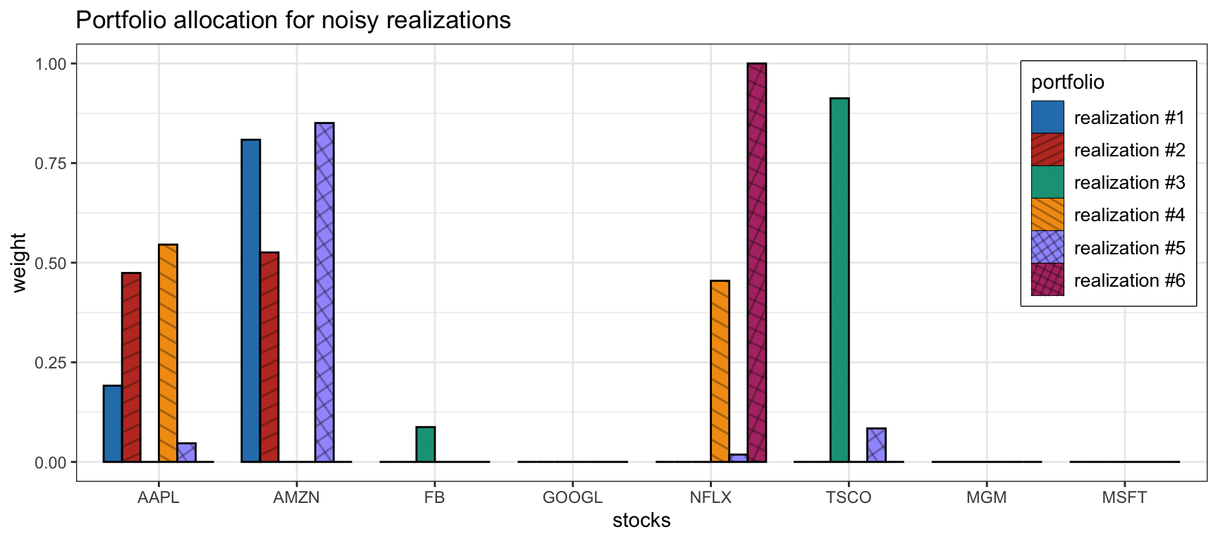
Figure 7.9: Effect of parameter estimation noise in the MVP allocation.
This motivates the pragmatic employment of the risk-based portfolios considered in Section 6.5, which do not make use of \(\bmu\) at all, or the use of the \(1/N\) portfolio introduced in Section 6.4.3. Alternatively, Section 7.1.5 explores several heuristic constraints that can help improve the practical performance of the otherwise unstable MVP. Indeed, as stated in Michaud (1989):
The major problem with MV optimization is its tendency to maximize the effects of errors in the input assumptions. Unconstrained MV optimization can yield results that are inferior to those of simple equal-weighting schemes.
There are at least two nonexclusive ways to attempt to fix this problem of the noise in the estimated parameters \(\bmu\) and \(\bSigma\) and its effect in the portfolio: improved estimators and robust optimization. One way is by improving the estimation process to reduce the noise as explored in Chapter 3. This includes the use of prior information in the Black–Litterman framework or via shrinkage, as well as employing better statistical models for the data such as heavy-tailed distributions (as opposed to the Gaussian or normal distribution). Another way is to embrace the fact that the parameters contain noise and employ statistical techniques such as bootstrapping or resampling, as well as the more sophisticated robust optimization techniques explored in Chapter 14.
7.5.2 Variance or Volatility as Measure of Risk
In Markowtiz’s mean–variance portfolio, the risk is measured by the variance or, equivalently, by the volatility (Markowitz, 1952). The rationale is that a higher variance means that there are large peaks in the return distribution which may cause big losses. However, Markowitz himself already recognized and stressed the limitations of mean–variance analysis (Markowitz, 1959).
To start with, the variance is not a good measure of risk in practice since it penalizes both the unwanted losses and the desired negative losses (i.e., positive gains). Indeed, the mean–variance portfolio framework penalizes up-side and down-side risk equally, whereas most investors do not mind up-side risk. In addition, the variance only measures the width of the main mode of the probability distribution, whereas the most critical part lies in the tail of big losses (see Figure 6.10). The solution is to use alternative measures for risk such as downside risk, semi-variance, VaR, CVaR, and drawdown (McNeil et al., 2015); see Section 6.3.
Chapter 10 explores portfolio formulations under alternative risk measures such as downside risk, semi-variance, VaR, CVaR, and drawdown.
7.5.3 Single-Number Measure of Risk
Regardless of the choice of risk measure (i.e., variance, volatility, downside risk, semi-variance, VaR, CVaR, or worst drawdown), the risk of the portfolio is measured by a single number. This risk characterization may not be enough to properly understand the risk contribution from the different assets, which leads us to the concept of risk diversification to avoid concentration of risk into a few assets (e.g., as was observed during the 2008 financial crisis).
Particularly, the risk parity portfolio, considered in Chapter 11, delves into the decomposition of the overall risk into contributions from each of the assets (Qian, 2005) and allows proper risk diversification.