\( \newcommand{\bm}[1]{\boldsymbol{#1}} \newcommand{\textm}[1]{\textsf{#1}} \def\T{{\mkern-2mu\raise-1mu\mathsf{T}}} \newcommand{\R}{\mathbb{R}} % real numbers \newcommand{\E}{{\rm I\kern-.2em E}} \newcommand{\w}{\bm{w}} % bold w \newcommand{\bmu}{\bm{\mu}} % bold mu \newcommand{\bSigma}{\bm{\Sigma}} % bold mu \newcommand{\bigO}{O} %\mathcal{O} \renewcommand{\d}[1]{\operatorname{d}\!{#1}} \)

2.3 Non-Gaussianity: Asymmetry and heavy tails

The Gaussian or normal distribution is one of the most commonly used for continuous random variables due to its ease of mathematical manipulation. It is characterized by two parameters: the mean and the variance (first- and second-order moments). Its probability distribution function (pdf) reads: \[ f(x) = \frac{1}{\sqrt{2\pi}\sigma} e^{-\frac{1}{2}\left(\frac{x - \mu}{\sigma}\right)^2}, \] where \(\mu\) is the mean and \(\sigma^2\) is the variance.

In many areas, the Gaussian distribution may in fact be appropriate and easily justified from physical principles (like the pervasive thermal noise in electronic circuits that hinders communication systems). However, in other domains, like radar and financial systems, the random quantities are often not Gaussian distributed and higher-order moments are necessary for a proper characterization (Jondeau et al., 2007). Two new aspects enter the picture for a proper characterization:

• the skewness as a measure of the asymmetry in the distribution, and
• the kurtosis as a measure of the thickness of the tails (i.e., whether the tails decay faster or slower than the exponential decay of the Gaussian distribution).

Figure 2.6 illustrates the effect of skewness and kurtosis on the pdf. Financial data typically exhibits negative skewness and large kurtosis (with potential huge losses due to the left heavy tail).

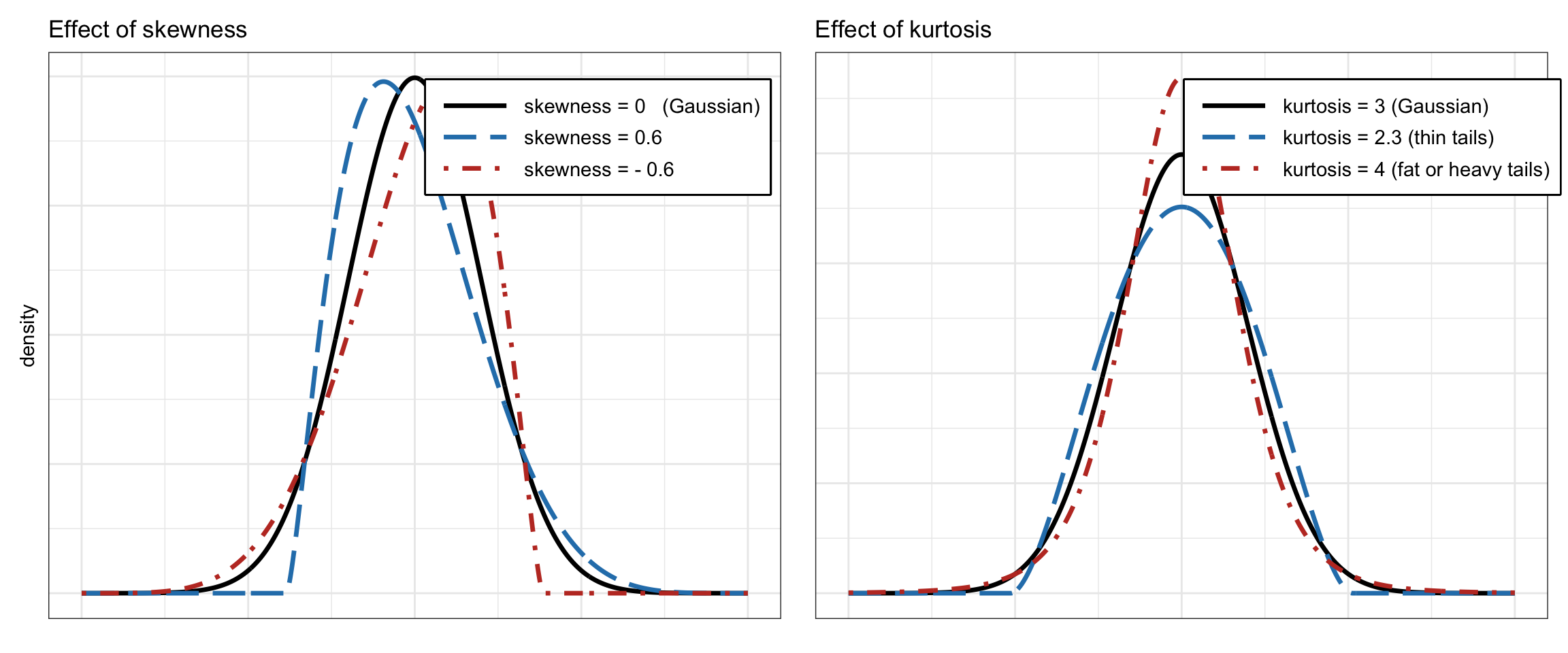
Figure 2.6: Effect of skewness and kurtosis on the probability distribution function.

The combination of skewness and kurtosis makes it more likely for highly negative returns to occur (with the obvious consequences for an investor who has bought the asset). This is illustrated in Figure 2.7, where the left tail of a typical distribution of financial data is clearly shown to be much fatter or heavier than that of a Gaussian distribution. This is why distributions with tails decaying slower than the exponential (decay of the Gaussian) are called heavy tails, fat tails, or thick tails.

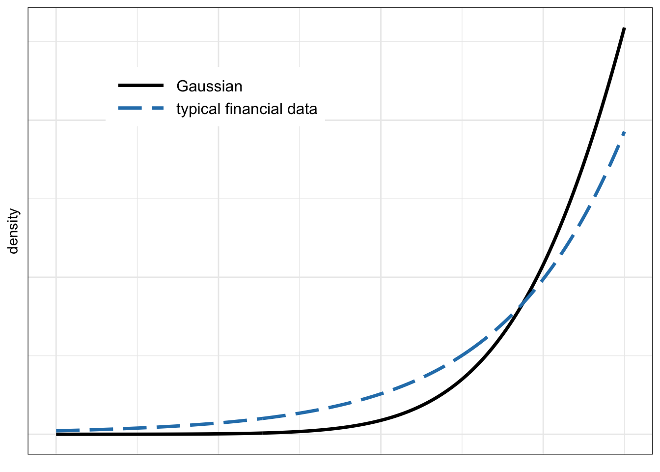
Figure 2.7: Left tail of Gaussian and typical financial data distributions.

Figure 2.8 shows the histogram of the S&P 500 log-returns at different frequencies (namely, daily, monthly, and quarterly). It can be seen that the tails of the histogram are significantly heavier or thicker than that of a Gaussian and that the histogram is not symmetric. Figure 2.9 shows the histogram of Bitcoin log-returns, again with clear heavy tails, although the asymmetry seems less pronounced than in the S&P 500 case.

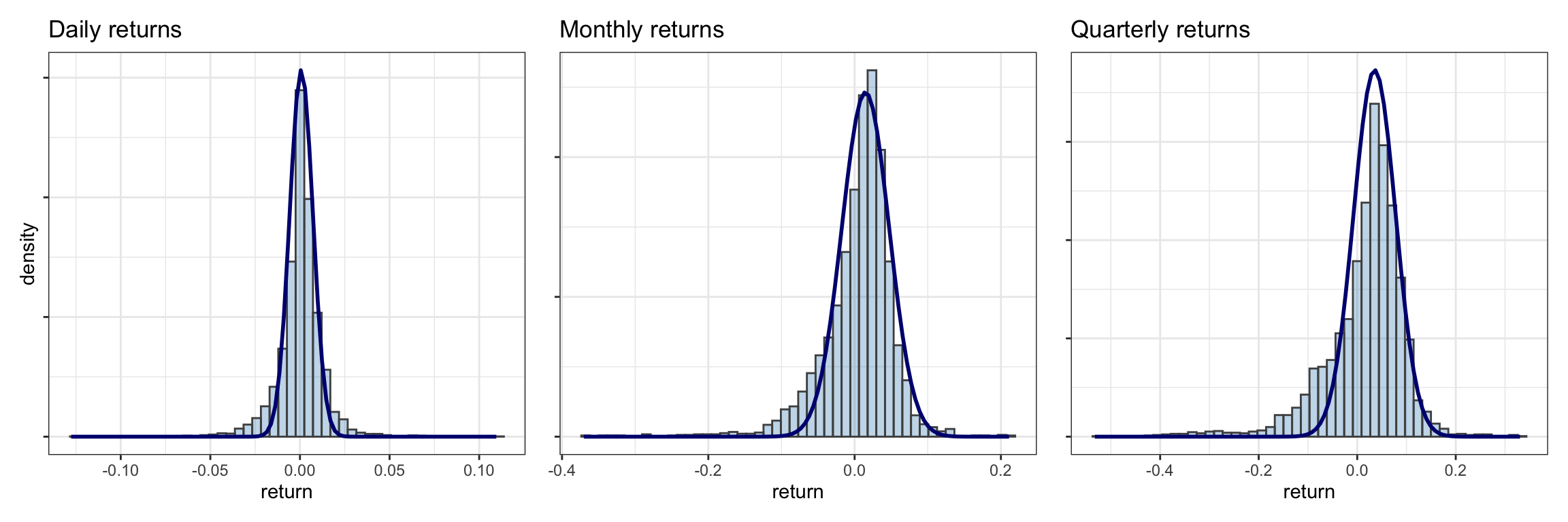
Figure 2.8: Histogram of S&P 500 log-returns at different frequencies (with inappropriate Gaussian fit).

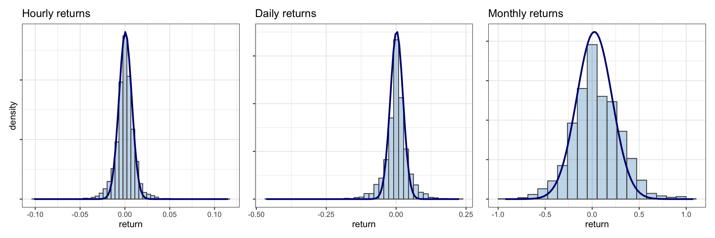
Figure 2.9: Histogram of Bitcoin log-returns at different frequencies (with inappropriate Gaussian fit).

While the histograms provide a quick visual inspection of the whole distribution, there are other more convenient type of plots that allow for a clearer characterization of the level of asymmetry and heavy-tailness.

Asymmetry or skewness

Skewness is a measure of the asymmetry of the probability distribution of a real-valued random variable about its mean. Zero skewness implies a symmetric distribution, negative skew commonly indicates that the thick tail is on the left side of the distribution, whereas positive skew indicates that the thick tail is on the right. The skewness of a random variable \(X\) is defined as the third standardized moment \(\E\left[\left(\frac{X - \mu}{\sigma}\right)^3\right]\).

Figure 2.10 plots the skewness of the S&P 500 returns during 2007-2022 as a function of the period of the returns. As the period increases from one day to ten days, the skewness decreases rapidly; then it saturates. Figure 2.11 shows the same for Bitcoin during 2017-2022, with similar results. As previously observed from the histograms, the skewness of Bitcoin is closer to zero than that of the S&P 500. Thus, as a first approximation, cryptocurrencies seem to be more symmetric than stocks.

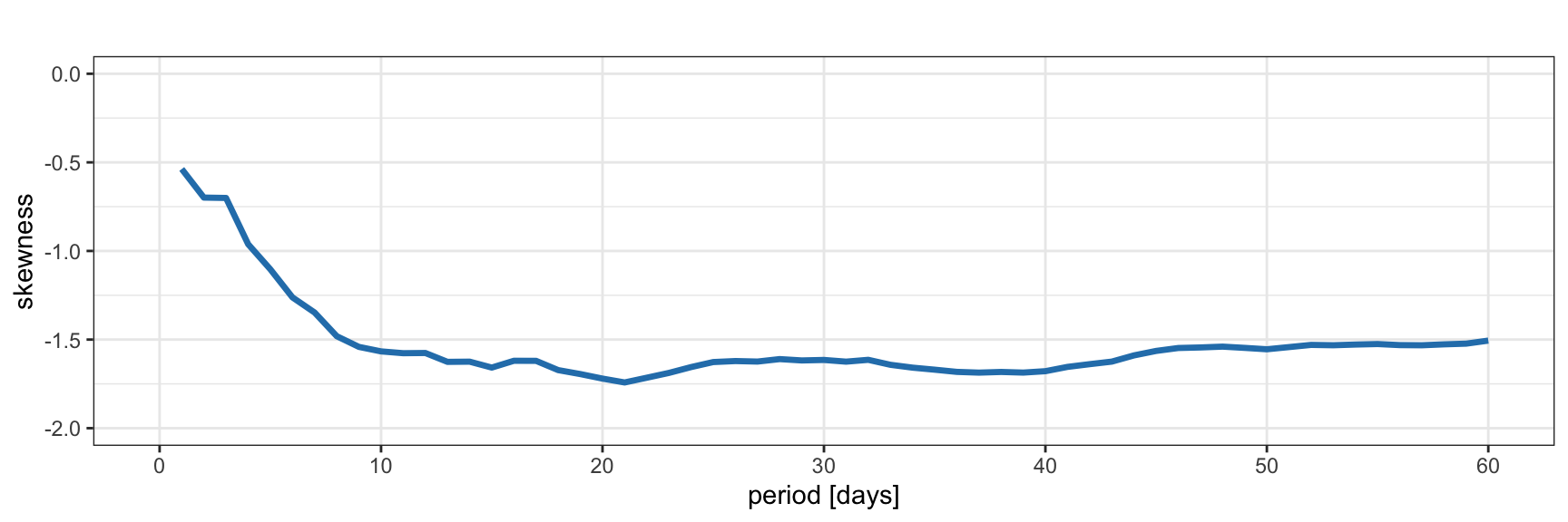
Figure 2.10: Skewness of S&P 500 log-returns.

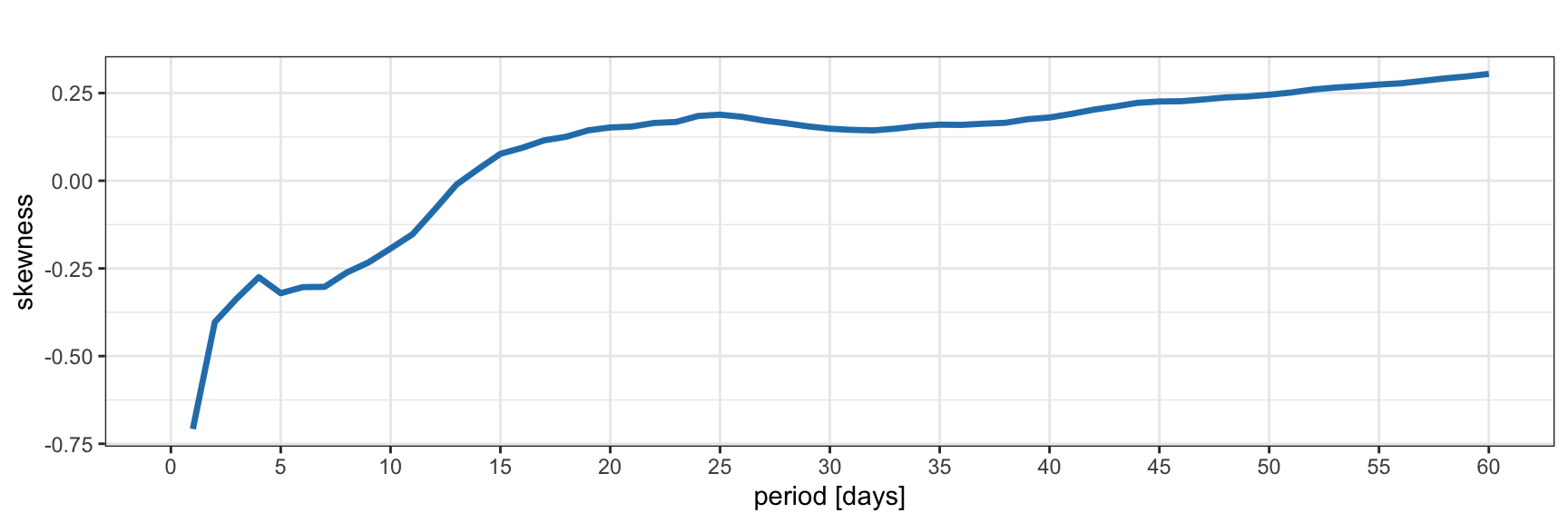
Figure 2.11: Skewness of Bitcoin log-returns.

Heavy-tailness or kurtosis

Q-Q (quantile-quantile) plots allow for a clearer assessment of the degree of heavy tails as compared to the exponential one of the Gaussian case. Figures 2.12 and 2.13 show Q-Q plots corresponding to the S&P 500 and Bitcoin log-returns, respectively. The deviation of both the left and right tails in all cases clearly indicates heavy tails.

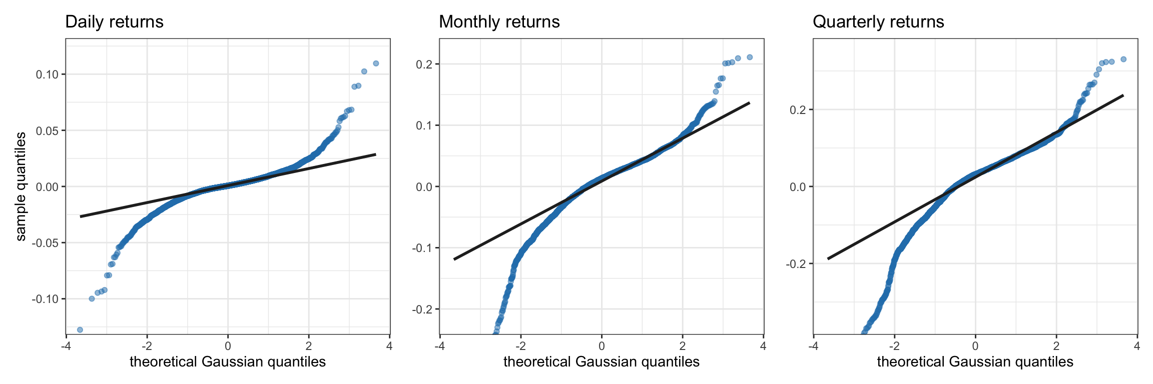
Figure 2.12: Q-Q plots of S&P 500 log-returns at different frequencies.

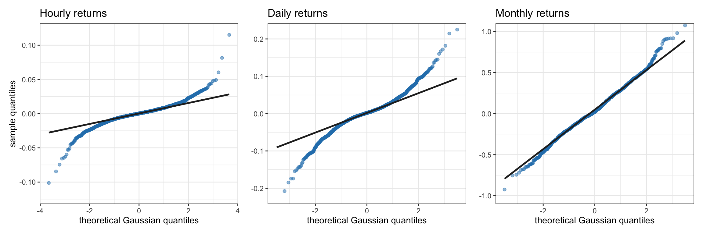
Figure 2.13: Q-Q plots of Bitcoin log-returns at different frequencies.

Kurtosis is a measure of the “tailedness” or “tail heavyness” of the probability distribution of a real-valued random variable. Like skewness, kurtosis describes the shape of a probability distribution and there are different ways of quantifying it. The kurtosis of a Gaussian distribution is 3. Higher kurtosis values corresponds to greater extremity of deviations (or outliers), hence the names heavy/fat/thick tails. It is common practice to use an adjusted version of the kurtosis, the excess kurtosis, which is the kurtosis minus 3. The standard definition of the kurtosis of a random variable \(X\) is the fourth standardized moment \(\E\left[\left(\frac{X - \mu}{\sigma}\right)^4\right]\).

Figure 2.14 plots the kurtosis of the S&P 500 returns during 2007-2022 as a function of the period of the returns. As the period increases from one day to three days, the excess kurtosis decreases very rapidly and then it saturates around 6 to 8. Similarly, Figure 2.15 shows the kurtosis of Bitcoin returns during 2017-2022. As the period increases from one to three days, the excess kurtosis decreases very rapidly to less then 3. Interestingly, the kurtosis of Bitcoin seems to be smaller than that of the S&P 500. Thus, as a first approximation, it may seem that cryptocurrencies are less heavy-tailed or more Gaussian than stocks. However, this deserves a closer look by looking at the excess kurtosis during different periods:

• From 2017 to 2019: 5.41 for the S&P 500 and 3.46 for Bitcoin.
• During 2020: 8.51 for the S&P 500 and 50.87 for Bitcoin.
• From 2021 to 2022: 0.95 for the S&P 500 and 2.34 Bitcoin.

From these distinct periods, it is evident that the primary difference occurred in 2020, during which Bitcoin exhibited significantly more heavy-tailed behavior.

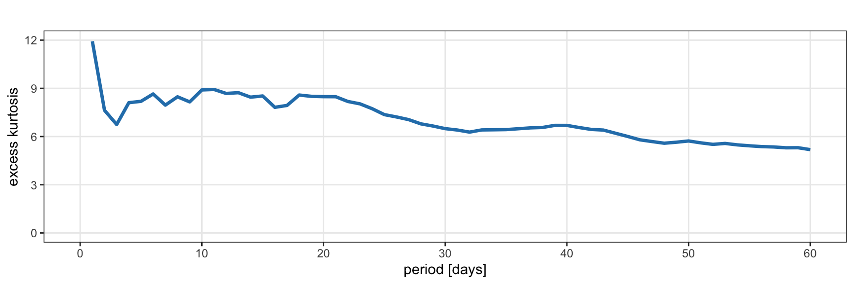
Figure 2.14: Excess kurtosis of S&P 500 log-returns.

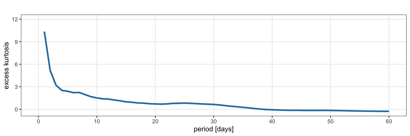
Figure 2.15: Excess kurtosis of Bitcoin log-returns.

Statistical tests

From the previous analysis, financial data clearly show skewness and kurtosis. To assess whether these parameters, together with the mean and variance, are enough to characterize the data, we can resort to mathematical sound statistical tests.

The Anderson–Darling statistic measures how well the data follow a particular distribution (the better the distribution fits the data, the smaller this statistic will be). The hypotheses for the Anderson–Darling test are

• H0: the data follow a specified distribution (null hypothesis); and
• H1: the data do not follow a specified distribution (alternative hypothesis).

As customary, we can use the \(p\)-value to determine whether the data come from the chosen distribution (if it is smaller than some threshold, typically 0.05 or so, then we can reject the null hypothesis that the data came from that distribution).⁷

Table 2.1 shows the results of the Anderson–Darling test for three distributions: the Gaussian, the Student \(t\) distribution (which models heavy tails), and the skewed \(t\) distribution (which accounts for both skewness and heavy tails). From these results we can conclude that the skewed \(t\) distribution provides a good fit to the S&P 500 during the period 2015-2020. For an additional visual inspection, Figure 2.16 shows Q-Q plots of the empirical data with respect to the three candidate distributions (Gaussian, Student \(t\), and skewed \(t\)). We can again confirm that the skewed \(t\) distribution is a good fit.

Table 2.1: Results of Anderson–Darling test on financial data, suporting the skewed \(t\) distribution.

Distribution	Anderson-Darling test	\(p\)-value
Gaussian	55.315	4.17e-07
Student \(t\)	5.4503	0.001751
Skewed \(t\)	2.3208	0.06161

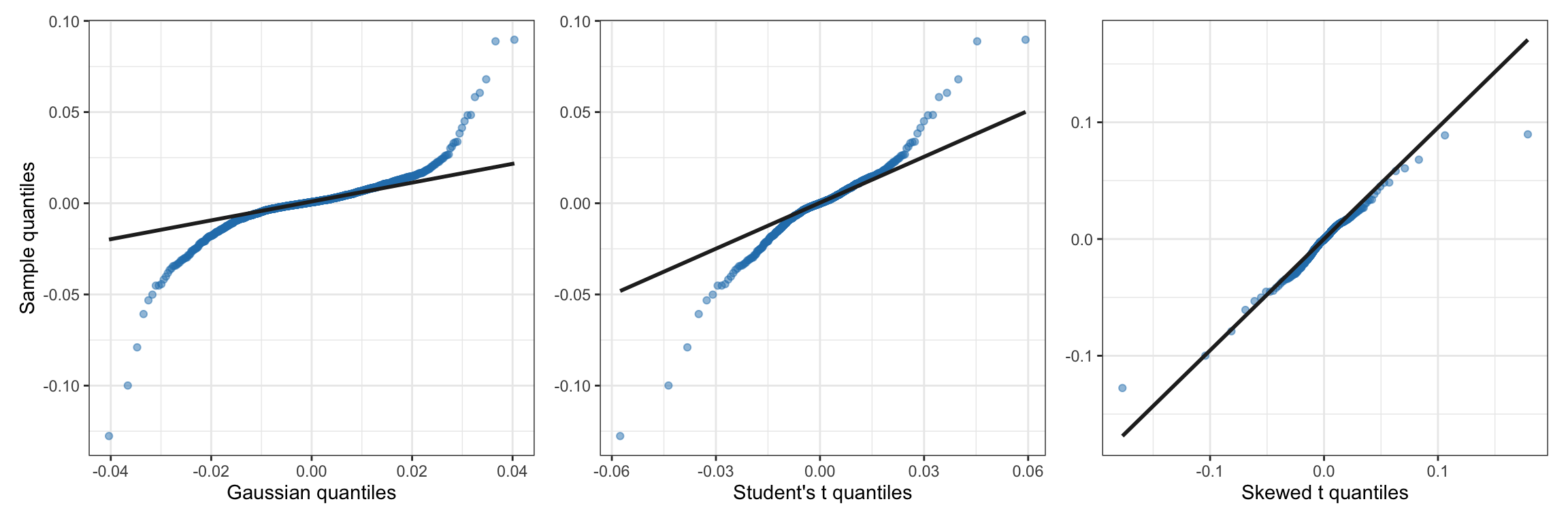
Figure 2.16: Q-Q plots of S&P 500 log-returns versus different candidate distributions.

References

Jondeau, E., Poon, S. H., and Rockinger, M. (2007). Financial modeling under non-Gaussian distributions. Springer.

---

7. The \(p\)-value is the probability of obtaining the observed results under the assumption that the null hypothesis is correct. A small \(p\)-value means that there is strong evidence to reject the null hypothesis and accept the alternative hypothesis. Typical thresholds for determining whether a \(p\)-value is small enough are in the range 0.01 - 0.05.↩︎