7.1 Mean–Variance Portfolio (MVP)
This section considers the mean–variance portfolio (MVP) proposed by Markowitz in his 1952 seminar paper (Markowitz, 1952); see also the monographs Rubinstein (2002) and Kolm et al. (2014) with a retrospective view.
7.1.1 Return–Risk Trade-Off
While the expected return of the portfolio \(\w^\T\bmu\) is a relevant quantity that measures the average or expected benefit (see Section 6.3), it leaves one key element out: the risk. An investor needs to control the probability of going bankrupt. A risk measure precisely quantifies how risky an investment strategy is. The most basic risk measure is the volatility \(\sqrt{\w^\T\bSigma\w}\) or, similarly, the variance \(\w^\T\bSigma\w\): a higher variance means that there are large peaks in the distribution of the returns, which may cause big losses. The volatility/variance has its limitations and a number of more sophisticated risk measures have been proposed in the literature such as downside risk measures (e.g., semi-variance), VaR, and CVaR (see Section 6.3).
Precisely, Markowitz put forth the idea that risk-adverse investors should optimize their portfolio based on a combination of two objectives: expected return and risk (Markowitz, 1952). However, there is a trade-off between these two objectives: the higher the expected return, the higher the risk; the lower the risk, the lower the expected return. In other words, we are dealing with a multi-objective optimization problem (see Section A.7 in Appendix A) with its corresponding optimal trade-off curve (Pareto-optimal points), which is called the efficient frontier in this portfolio context. Basically, the efficient frontier is a curve representing the best possible pair values of expected return and volatility that can be achieved by any feasible portfolio. The choice of a specific point on this trade-off curve depends on how aggressive or risk-averse the investor is. Figure 7.1 shows the trade-off between expected return and volatility.
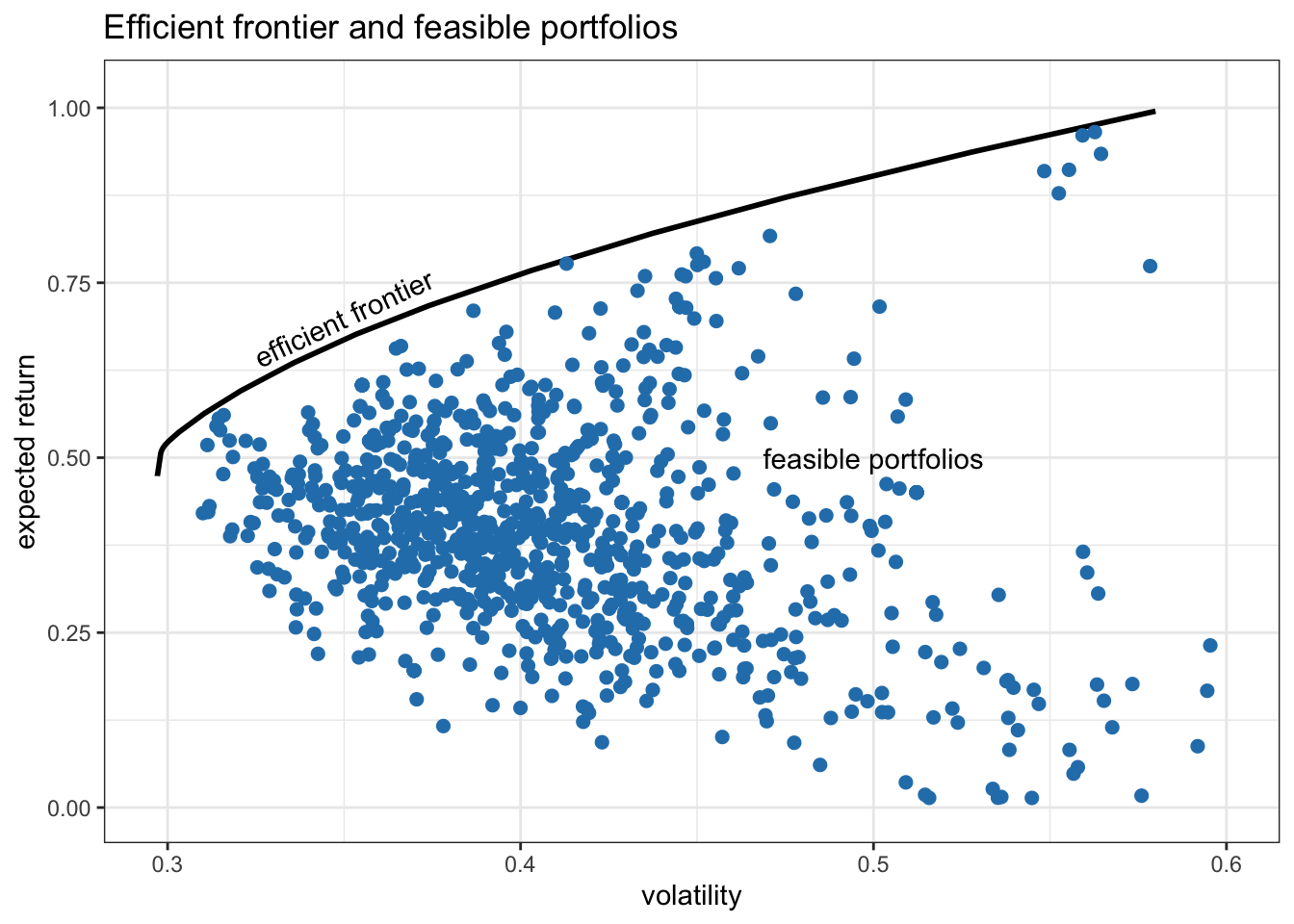
Figure 7.1: Trade-off between expected return and volatility: efficient frontier and 1,000 random feasible portfolios.
7.1.2 MVP Formulation
Markowitz’s portfolio formulation is a bi-objective optimization problem with the two objectives being the expected return \(\w^\T\bmu\) and the risk measured by the volatility \(\sqrt{\w^\T\bSigma\w}\) or, similarly, the variance \(\w^\T\bSigma\w\). From an algorithmic perspective, it is more computationally efficient to use the variance than the volatility, since the former involves quadratic programming whereas the latter results in second-order cone programming (see Appendix A and, more specifically, Section B.1 in Appendix B for algorithmic aspects of solvers).
There are several ways to formulate a bi-objective optimization problem, as discussed in Section A.7. The most convenient way is via scalarization of the two objectives into a single objective with a weighted sum (Markowitz, 1952): \[\begin{equation} \begin{array}{ll} \underset{\w}{\textm{maximize}} & \w^\T\bmu - \frac{\lambda}{2}\w^\T\bSigma\w\\ \textm{subject to} & \bm{1}^\T\w=1, \quad \w\ge\bm{0}, \end{array} \tag{7.1} \end{equation}\] where \(\lambda\) is a hyper-parameter that controls how risk-averse the investor is. The two constraints included are just for illustration purposes; in practice, one can include many of the other constraints listed in Section 6.2, as elaborated in Section 7.1.4.
The choice of \(\lambda\) in the MVP in (7.1) will produce different portfolios that lie along the efficient frontier shown in Figure 7.2. In fact, by letting \(\lambda\) vary from \(0\) to \(\infty\), one can recover the whole efficient frontier. In particular, for \(\lambda=0\) we recover the global maximum return portfolio (GMRP) described in Section 6.4.2 (i.e., only the expected return is considered while the variance is ignored), whereas for \(\lambda \rightarrow \infty\) we recover the global minimum variance portfolio (GMVP) considered in Section 6.5.1 (i.e., the expected return is not used at all). Figure 7.2 shows the efficient frontier together with these portfolios.
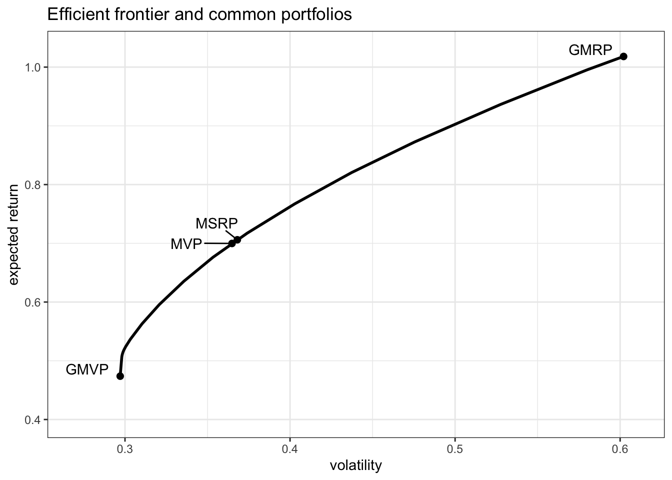
Figure 7.2: Efficient frontier and common portfolios.
Problem (7.1) is a quadratic problem (QP) that can be easily solved with a QP solver (see Appendix B). If we ignore the no-shorting constraint \(\w\ge\bm{0}\), then the problem admits the simple closed-form solution \[ \w = \frac{1}{\lambda} \bSigma^{-1}\left(\bmu + \nu\bm{1}\right), \] where \(\nu\) is the optimal dual variable \(\nu=\frac{\lambda-\bm{1}^{\T}\bSigma^{-1}\bmu}{\bm{1}^{\T}\bSigma^{-1}\bm{1}}\) chosen to satisfy the normalization constraint \(\bm{1}^\T\w=1\).
Example 7.1 (Optimum investment sizing) Suppose we have a single asset or a fully invested portfolio (\(\bm{1}^\T\w=1\)) with some returns over time \(r_1, r_2, \dots\) The problem of investment sizing refers to determining how much of the budget should be allocated to this risky asset and how much should be kept in cash. The optimal sizing can be obtained from the MVP formulation in (7.1) particularized to \(N=1\) as \[ \begin{array}{ll} \underset{w}{\textm{maximize}} & w\mu - \frac{\lambda}{2}w^2\sigma^2\\ \textm{subject to} & 0 \le w \le 1, \end{array} \] with solution \[ w = \left[ \frac{1}{\lambda} \frac{\mu}{\sigma^2} \right]_0^1, \] where \([\cdot]_0^1\) denotes projection on the interval \([0,1]\). In particular, the growth rate is maximized when \(\lambda=1\) (see Section 7.3.1 for details) and then the optimal sizing turns out to be the (projected) mean-to-variance ratio: \(w=[\mu/\sigma^2]_0^1\).
There are two other widely used reformulations of Markowitz’s portfolio. One formulation has the variance term as a constraint: \[\begin{equation} \begin{array}{ll} \underset{\w}{\textm{maximize}} & \w^\T\bmu\\ \textm{subject to} & \w^\T\bSigma\w \leq \alpha,\\ & \bm{1}^\T\w=1, \quad \w\ge\bm{0}, \end{array} \tag{7.2} \end{equation}\] where \(\alpha\) is a hyper-parameter that controls the maximum level of variance accepted. The other formulation, instead, has the expected return as a constraint: \[\begin{equation} \begin{array}{ll} \underset{\w}{\textm{minimize}} & \w^\T\bSigma\w\\ \textm{subject to} & \w^\T\bmu \geq \beta,\\ & \bm{1}^\T\w=1, \quad \w\ge\bm{0}, \end{array} \tag{7.3} \end{equation}\] where \(\beta\) is a hyper-parameter that controls the minimum level of expected return accepted.
Similarly to what happens with formulation (7.1) as the hyper-parameter \(\lambda\) is varied, formulations (7.2) and (7.3) can also recover the whole efficient frontier by changing the hyper-parameters \(\alpha\) and \(\beta\), respectively.
The hyper-parameters in formulations (7.2) and (7.3) have a more intuitive interpretation than that in formulation (7.1), that is, maximum accepted variance and minimum accepted expected return. On the other hand, formulations (7.2) and (7.3) may be infeasible if the hyper-parameters are not properly chosen, whereas formulation (7.1) is always feasible regardless of the hyper-parameter \(\lambda\). To avoid running into infeasibility issues, it is customary to choose the hyper-parameters based on benchmark portfolios such as the \(1/N\) portfolio, i.e., \(\alpha = \frac{1}{N^2}\bm{1}^\T\bSigma\bm{1}\) or \(\beta = \frac{1}{N}\bm{1}^\T\bmu\).
Problem (7.3) is still a QP that can be solved efficiently with a QP solver; however, problem (7.2) is a quadratically-constrained QP (QCQP) which typically requires a higher complexity either by using a QCQP solver or an SOCP solver (see Section B.1 for details).
Commonly used programming languages in finance offer packages specifically designed to optimize portfolios under a wide variety of formulations and constraints, such as the popular R package fPortfolio (Wuertz et al., 2023) and the Python library Riskfolio-Lib (D. Cajas, 2023).
Figure 7.3 shows the portfolio allocation of the MVP in (7.1) for different values of \(\lambda\), from which we can see the critical effect of the hyper-parameter in the final allocation. Figure 7.4 and Table 7.1 show the corresponding backtest results, indicating that smaller values of \(\lambda\) suffer from a worse Sharpe ratio and a much severe drawdown than the largest ones.
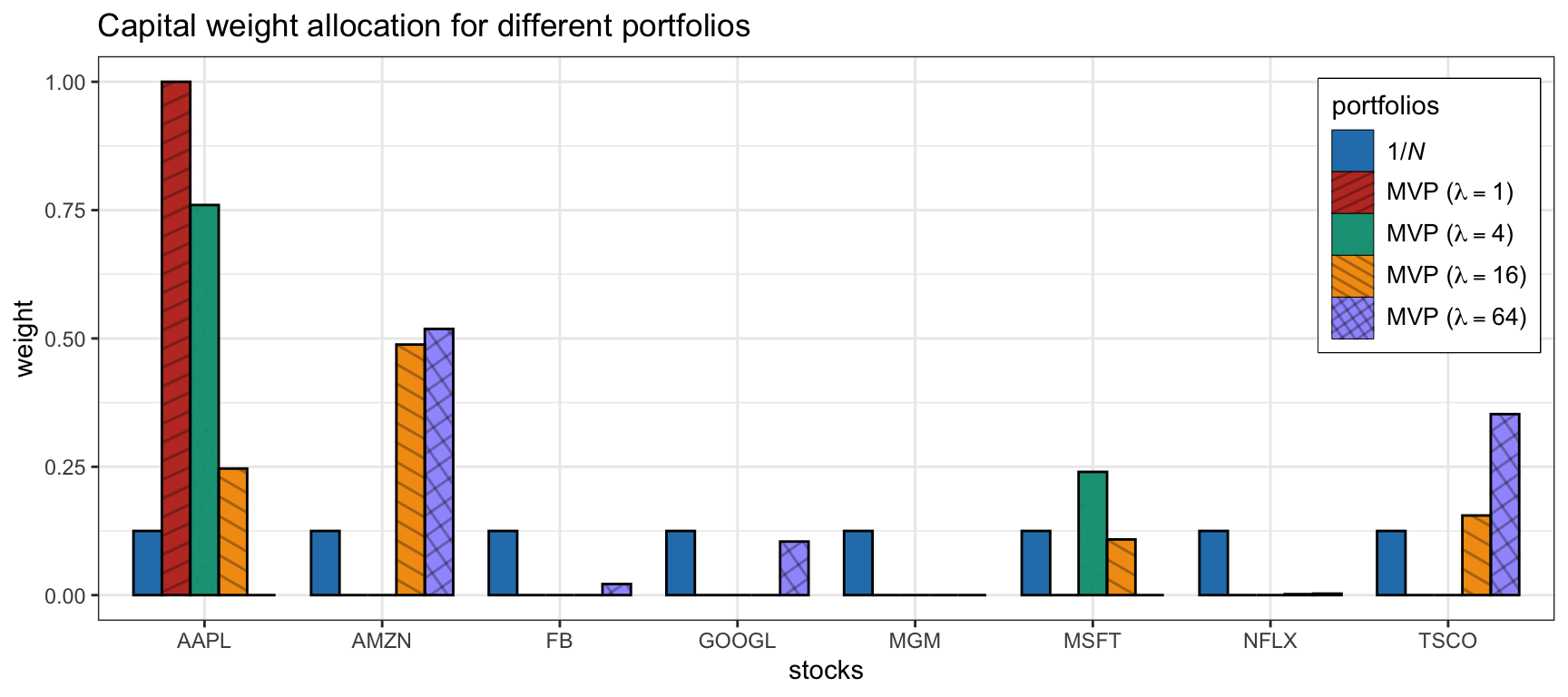
Figure 7.3: Portfolio allocation of MVP with different values of hyper-parameter \(\lambda\).
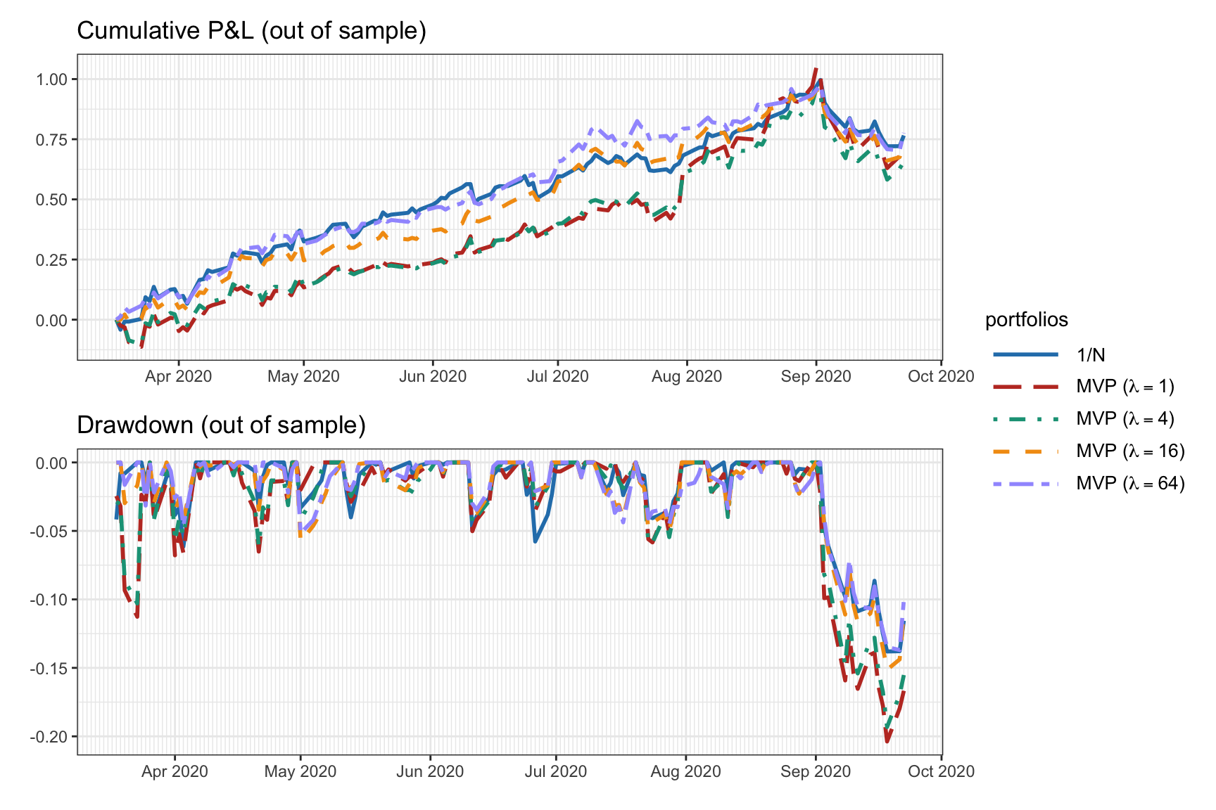
Figure 7.4: Backtest performance of MVP with different values of hyper-parameter \(\lambda\).
| Portfolio | Sharpe ratio | Annual return | Annual volatility | Max drawdown |
|---|---|---|---|---|
| \(1/N\) | 3.34 | 115% | 35% | 14% |
| MVP (\(\lambda = 1\)) | 2.60 | 112% | 43% | 20% |
| MVP (\(\lambda = 4\)) | 2.57 | 106% | 41% | 19% |
| MVP (\(\lambda = 16\)) | 3.37 | 113% | 33% | 15% |
| MVP (\(\lambda = 64\)) | 3.65 | 116% | 32% | 14% |
7.1.3 MVP as a Regression
Interestingly, the MVP formulation can be interpreted as a regression problem. The key observation is that the variance of the portfolio can be seen as an \(\ell_2\)-norm error term. First, we rewrite the variance as \[ \begin{aligned} \w^\T\bSigma\w &= \w^\T\E\left[(\bm{r}_t-\bmu)(\bm{r}_t-\bmu)^\T\right]\w\\ &= \E\left[(\w^\T(\bm{r}_t-\bmu))^2\right]\\ &= \E\left[(\w^\T\bm{r}_t-\rho)^2\right], \end{aligned} \] where \(\rho = \w^\T\bmu\). Then, we use the sample approximation for the expected value, \[ \E\left[(\w^\T\bm{r}_t - \rho)^2\right] \approx \frac{1}{T}\sum_{t=1}^T (\w^\T\bm{r}_t - \rho)^2 = \frac{1}{T}\|\bm{R}\w - \rho\bm{1}\|_2^2, \] where \(\bm{R} \triangleq \left[\bm{r}_1,\dots,\bm{r}_T \right]^\T\).
Now we can continue by rewriting the MVP formulation (7.1) as the minimization \[ \begin{array}{ll} \underset{\w}{\textm{minimize}} & \w^\T\bSigma\w - \frac{2}{\lambda}\w^\T\bmu\\ \textm{subject to} & \bm{1}^\T\w=1, \quad \w\ge\bm{0} \end{array} \] and finally substitute the variance with the \(\ell_2\)-norm expression: \[\begin{equation} \begin{array}{ll} \underset{\w,\rho}{\textm{minimize}} & \frac{1}{T}\|\bm{R}\w - \rho\bm{1}\|_2^2 - \frac{2}{\lambda}\rho\\ \textm{subject to} & \rho = \w^\T\bmu,\\ & \bm{1}^\T\w=1, \quad \w\ge\bm{0}. \end{array} \tag{7.4} \end{equation}\] Note that the expected return, denoted by \(\rho\), is also an optimization variable. Alternatively, one could fix \(\rho\) to some predetermined value.
From the MVP formulation as a regression in (7.4), we can interpret the portfolio \(\w\) as trying to obtain returns over time as constant as possible and equal to \(\rho\). In other words, it is trying to achieve or track the expected return \(\rho\) with minimum variance as measured by the \(\ell_2\)-norm. Interestingly, this interpretation is in fact related to the topic of index tracking in Chapter 13.
7.1.4 MVP with Practical Constraints
The previous MVP formulations in (7.1), (7.2), and (7.3) have included the two simple constraints \(\bm{1}^\T\w=1\) and \(\w\ge\bm{0}\) for simplicitly of exposition. In practice, however, there is a multitude of other constraints that an investor may want to use, as listed in Section 6.2; see also Kolm et al. (2014).
For example, we can start with the basic MVP formulation in (7.1) that only contains the budget and no-shorting constraints, \[ \begin{array}{ll} \underset{\w}{\textm{maximize}} & \begin{array}{l}\w^\T\bmu - \frac{\lambda}{2}\w^\T\bSigma\w\end{array}\\ \textm{subject to} & \begin{array}[t]{ll} \bm{1}^\T\w=1 & \textm{budget},\\ \w\ge\bm{0} & \textm{no-shorting}, \end{array} \end{array} \] and change the constraints to reflect a more realistic trading situation: \[\begin{equation} \begin{array}{ll} \underset{\w}{\textm{maximize}} & \begin{array}{l}\w^\T\bmu - \frac{\lambda}{2}\w^\T\bSigma\w\end{array}\\ \textm{subject to} & \begin{array}[t]{ll} \left\Vert \w\right\Vert_1\leq\gamma & \textm{leverage},\\ \left\Vert \w-\w_{0}\right\Vert _{1}\leq\tau & \textm{turnover},\\ |\w| \leq \bm{u} & \textm{max positions},\\ \bm{\beta}^\T\w = 0 & \textm{market neutral},\\ \left\Vert \w\right\Vert _{0} \leq K & \textm{sparsity}, \end{array} \end{array} \tag{7.5} \end{equation}\] where \(\gamma\geq1\) controls the amount of shorting and leverage, \(\tau>0\) controls the turnover (to limit the transaction costs in the rebalancing), \(\bm{u}\) limits the position in each stock, \(\bm{\beta}\) denotes the beta of the stocks, and \(K\) controls the cardinality of the portfolio (to select a small set of stocks from the universe).
More generally, we can write the MVP formulation with a general set of constraints, denoted by \(\mathcal{W}\), as \[\begin{equation} \begin{array}{ll} \underset{\w}{\textm{maximize}} & \w^\T\bmu - \frac{\lambda}{2}\w^\T\bSigma\w\\ \textm{subject to} & \w \in \mathcal{W}. \end{array} \tag{7.6} \end{equation}\]
From the optimization perspective, as long as the constraints in \(\mathcal{W}\) are convex the problem will remain convex and will still be easy to solve. The only constraint that is nonconvex in (7.5) is the cardinality constraint \(\left\Vert \w\right\Vert _{0} \leq K\).
7.1.5 Improving the MVP with Heuristics
One of the main problems of the MVP is the lack of diversification, which goes against common practice. To address this issue, several heuristics have been proposed with good practical results such as no-shorting constraints, upper bound constraints, and \(\ell_2\)-norm constraints; see Kolm et al. (2014) for more details.
Imposing no-shorting constraints, \(\w\ge\bm{0}\), seems to have significant practical benefits in reducing the amplification of the noise inherent in the estimated covariance matrix, even when the constraints are wrong (Jagannathan and Ma, 2003). Surprisingly, with no-shorting constraints, the sample covariance matrix performs as well as more sophisticated covariance matrix estimators based on factor models, shrinkage estimators, or higher-frequency returns. Including upper bound constraints also has a regularization effect on the covariance matrix.
For example, if we consider the GMVP from Section 6.5.1 with constraints \(\bm{1}^\T\w=1\) and \(\bm{0}\leq\w\leq\bm{u}\), the optimal solution (6.15) is still valid using instead the regularized covariance matrix \[ \tilde{\bSigma} = \bSigma + \bm{\lambda}_0\bm{1}^\T + \bm{1}\bm{\lambda}_0^\T + \bm{\lambda}_{\textm{u}}\bm{1}^\T + \bm{1}\bm{\lambda}_{\textm{u}}^\T, \] where \(\bm{\lambda}_0\) and \(\bm{\lambda}_{\textm{u}}\) are the Lagrange multipliers corresponding to the no-shorting and upper bound constraints, respectively (Jagannathan and Ma, 2003). This regularized covariance matrix \(\tilde{\bSigma}\) can be interpreted as a shrunk version of \(\bSigma\) with reduced sampling error. Interestingly, the same result can be obtained by instead including an \(\ell_1\)-norm constraint \(\|\w\|_1\leq\delta\) (DeMiguel, Garlappi, Nogales, et al., 2009).
One way to enforce diversity is via the diversification constraint \(\|\w\|_2^2 \leq D\) (see Section 6.2). The maximum diversity level \(D\) is lower bounded by \(1/N\) (achieved by the \(1/N\) portfolio) and could be chosen as the diversity achieved by some benchmark portfolio, for example, the GMVP gives \(D = \bm{1}^\T\bSigma^{-2}\bm{1}/(\bm{1}^\T\bSigma^{-1}\bm{1})^2\).
For example, if we consider the GMVP with constraints \(\bm{1}^\T\w=1\) and \(\|\w\|_2^2 \leq D\), the optimal solution (6.15) is still valid using instead the regularized covariance matrix \[ \tilde{\bSigma} = \bSigma + \gamma\bm{I}, \] leading to the portfolio \[ \w = \frac{1}{\bm{1}^\T\left(\bSigma+\gamma\bm{I}\right)^{-1}\bm{1}} \left(\bSigma+\gamma\bm{I}\right)^{-1}\bm{1}, \] where \(\gamma\ge0\) is the Lagrange multiplier corresponding to the diversification constraint (DeMiguel, Garlappi, Nogales, et al., 2009). For \(\gamma=0\) we recover the solution (6.15), whereas for \(\gamma\rightarrow\infty\) we obtain the \(1/N\) portfolio. Interestingly, this solution is like shrinking the covariance matrix to the identity matrix with \(\gamma\) being the shrinkage intensity (see Chapter 3).
Figure 7.5 illustrates the effect of two diversification heuristics on the portfolio allocation (namely, with upper bound \(\|\w\|_\infty\leq0.25\) and diversification constraint \(\|\w\|_2^2\leq 0.25\)), which indeed improve the diversification. Figure 7.6 and Table 7.2 show the corresponding backtest results, indicating that the more diversified MVPs have a better Sharpe ratio and drawdown.
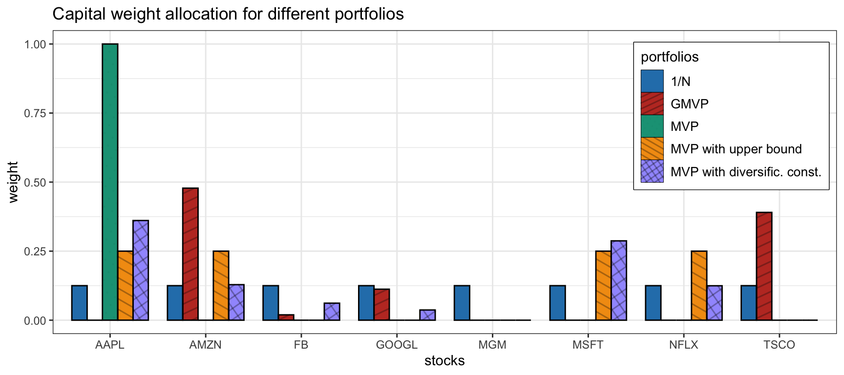
Figure 7.5: Portfolio allocation of MVP under two diversification heuristics (upper bound and diversification constraint).
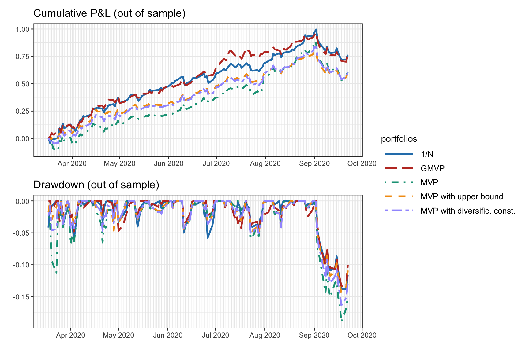
Figure 7.6: Backtest performance of MVP under two diversification heuristics (upper bound and diversification constraint).
| Portfolio | Sharpe ratio | Annual return | Annual volatility | Max drawdown |
|---|---|---|---|---|
| 1/\(N\) | 3.34 | 115% | 35% | 14% |
| GMVP | 3.67 | 115% | 31% | 14% |
| MVP | 2.44 | 99% | 41% | 19% |
| MVP with upper bound | 2.98 | 96% | 32% | 14% |
| MVP with diversific. const. | 2.79 | 97% | 35% | 16% |