4.1 Temporal Structure
From the exploratory analysis of financial data and stylized facts in Chapter 2, one can either assume the i.i.d. model, as pursued in detail in Chapter 3, or try to incorporate some temporal structure in the model, as this chapter attempts.
The i.i.d. model can be motivated by Fama’s efficient-market hypothesis (Fama, 1970), which holds that one cannot forecast future prices since the price of a security already contains all the publicly available information. On the other hand, an equally popular line of thought in finance supports inefficient and irrational markets (Shiller, 1981) under behavioral finance (Shiller, 2003).14 Under this premise, the market is predictable to some degree and perhaps it may move in trends so that the study of past prices can be used to forecast future price direction.
Thus, rather than assuming the random walk model (Malkiel, 1973), we will focus on nonrandom walk models (Lo and Mackinlay, 2002). Suppose we have \(N\) securities or tradable assets and let \(\bm{x}_t\in\R^N\) be the random returns of the assets at time \(t\). Instead of using the i.i.d. model for the returns, \(\bm{x}_t = \bmu + \bm{\epsilon}_t\) as in (3.1), we will now transition to a more general model in which the returns, \(\bm{x}_t\), are modeled conditioned on the past observations, denoted by \(\mathcal{F}_{t-1} \triangleq \{\dots,\bm{x}_{t-2},\bm{x}_{t-1}\}\), and then write \[\begin{equation} \bm{x}_t = \bmu_t + \bm{\epsilon}_t, \tag{4.1} \end{equation}\] where \(\bmu_t\in\R^N\) is the conditional expected return \[\bmu_t = \E\left[\bm{x}_t \mid \mathcal{F}_{t-1}\right]\] and \(\bm{\epsilon}_t\in\R^N\) denotes the error in the model (also called innovation or residual) with zero mean and conditional covariance matrix \[\bSigma_t = \E\left[(\bm{x}_t - \bmu_t)(\bm{x}_t - \bmu_t)^\T \mid \mathcal{F}_{t-1}\right].\]
The i.i.d. model in (3.1) from Chapter 3 can be obtained with the particular choice \(\bmu_t = \bmu\) and \(\bSigma_t = \bSigma\), which remain fixed over time.
Modeling the returns \(\bm{x}_t\) conditioned on the historical data \(\mathcal{F}_{t-1}\) is precisely one of the objectives in the field of econometrics, which integrates statistical and mathematical models to formulate theories or test existing hypotheses in economics, as well as to predict future trends based on historical data. Figure 4.1 shows an example of a synthetic univariate Gaussian AR(1) time series (model described later), where we can observe some temporal structure.
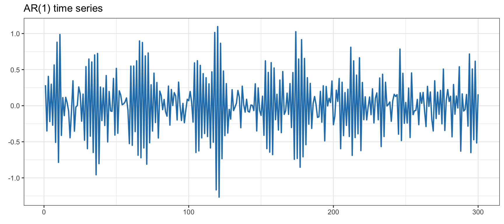
Figure 4.1: Example of a synthetic Gaussian AR(1) time series.
Some accessible textbooks that cover financial data modeling include Tsay (2010) and Ruppert and Matteson (2015), with more emphasis on the multivariate case in Lütkepohl (2007) and Tsay (2013). Some excellent survey papers are also available, such as Bollerslev et al. (1992), Taylor (1994), and Poon and Granger (2003).
This chapter deviates slightly from the conventional econometric modeling approaches, which typically revolve around autoregressive models and “GARCH” volatility models. Instead, the emphasis is placed on the simplicity of models combined with the versatile Kalman filter (often underutilized in financial literature, although still covered in Tsay (2010) and Lütkepohl (2007)). Additionally, stochastic volatility modeling is emphasized here, which frequently does not receive the attention it deserves in favor of more popular “GARCH” models. Specifically, after an introduction to Kalman filtering in Section 4.2, the following two families of models are presented:
References
It is somewhat interesting that both Robert J. Shiller and Eugene F. Fama were awarded the 2013 Sveriges Riksbank Prize in Economic Sciences in Memory of Alfred Nobel, when they support opposing views on the nature of financial markets, namely, the inefficiency of markets and the efficient-market hypothesis, respectively. ↩︎