15.4 Discovering Cointegrated Pairs
The key in pairs trading lies in being able to discover cointegrated pairs. The available methods range from simple heuristics to sophisticated multivariate modeling (Krauss, 2017).
15.4.1 Prescreening
Prescreening is a simple and cheap process by which many pairs can be easily discarded while some potential pairs are selected for further analysis. A common heuristic proxy for cointegration is the normalized price distance (NPD) defined as (Gatev et al., 2006) \[ \textm{NPD} \triangleq \sum_{t=1}^{T}\left(\tilde{p}_{1t} - \tilde{p}_{2t}\right)^{2}, \] where \(\tilde{p}_{1t}\) and \(\tilde{p}_{2t}\) are the normalized prices, \[ \begin{aligned} \tilde{p}_{1t} &= p_{1t}/p_{10},\\ \tilde{p}_{2t} &= p_{2t}/p_{20}, \end{aligned} \] with \(p_{1t}\) and \(p_{2t}\) being the original prices.
A similar distance measure can be defined in terms of log-prices, \(y_{1t}\) and \(y_{2t}\), by subtracting the initial value: \[ \begin{aligned} \tilde{y}_{1t} &= y_{1t} - y_{10},\\ \tilde{y}_{2t} &= y_{2t} - y_{20}. \end{aligned} \] Note that these shifted log-prices correspond to the long-term difference series, that is, the log-returns over long periods described earlier in Section 15.2 and denoted by \(r_{1t}(t)\) and \(r_{2t}(t)\).
15.4.2 Cointegration Tests
After the initial prescreening process of potential cointegrated pairs of assets, a more thorough analysis has to be performed. This is the job of the cointegration tests developed in the statistics literature for decades (Harris, 1995; Tsay, 2010, 2013). In a nutshell, these tests check whether or not a linear combination of the two time series follows a stationary autoregressive model and will be mean reverting. A time series with a unit root is nonstationary and behaves like a random walk. On the other hand, in the absence of unit roots, a time series tends to revert to its long-term mean. Thus, cointegration tests are typically implemented via unit-root stationarity tests.
Mathematically, we want to determine whether there exists a value of \(\gamma\) such that the spread \[ z_{t} = y_{1t} - \gamma \, y_{2t} \] is stationary. Note that, in practice, the mean of the spread \(\mu\) (equilibrium value) is not necessarily zero and \(\gamma\) does not have to be one. In fact, many studies artificially set \(\gamma=1\) to obtain dollar-neutral strategies (Elliott et al., 2005; Gatev et al., 2006; Triantafyllopoulos and Montana, 2011); however, that reduces the number of cointegrated pairs.
One of the simplest and most direct methods to test for cointegration is the Engle–Granger62 test (Engle and Granger, 1987). It is based on two steps: first, the value of \(\gamma\) is obtained via least squares regression, and then the residual is tested for stationarity.63 More exactly, the two sequences \(y_{1t}\) and \(y_{2t}\) are regressed against each other (see Chapter 3 for details on least squares regression), \[ y_{1t} - \gamma \, y_{2t} = \mu + r_t, \] and the residual \(r_t\) is checked for unit-root stationarity or some form of mean reversion.
There are many heuristic ways to measure the strength of the mean reversion of the residual. For example, one can use the mean-crossing rate, that is, the number of times the residual crosses its mean value over a period of time (Vidyamurthy, 2004): the higher the mean crossing rate, the stronger the mean reversion. Another measure is the half-life of the mean reversion (Chan, 2013), which quantifies the time it takes for a time series to return to within half of the distance from the mean after deviating a certain amount from the mean.
More formally, we can use mathematically well-defined statistical tests. A variety of such tests have been proposed over time, with some of the most popular ones being (A. Banerjee et al., 1993; Harris, 1995; Pfaff, 2008; Tsay, 2010, 2013):
- Dickey–Fuller (DF)
- augmented Dickey–Fuller (ADF)
- Phillips–Perron (PP)
- Pantula, Gonzales-Farias, and Fuller (PGFF)
- Elliott, Rothenberg, and Stock DF-GLS (ERSD)
- Johansen’s trace test (JOT)
- Schmidt and Phillips rho (SPR)
For example, the simplest model for the residual is \[ r_t = \rho \, r_{t-1} + \epsilon_t, \] where \(\epsilon_t\) is the innovation term, and stationarity requires no unit root in the autoregressive term, that is, \(|\rho| < 1\). The DF test (Dickey and Fuller, 1979) precisely formulates a hypothesis testing problem by defining the null hypothesis as a unit root being present (\(\rho=1\)) and the alternative hypothesis as the series being stationary (\(|\rho|<1\)). Under these two hypotheses, a small \(p\)-value64 indicates strong stationarity (rejection of the null hypothesis). The model for the residual can be extended to incorporate a constant and a linear trend: \[ r_t = \phi_0 + c\,t + \rho\,r_{t-1} + \epsilon_t. \] The popular ADF test includes further higher-order autoregressive terms in the model.
15.4.3 Cointegration of More Than Two Time Series
The Engle–Granger cointegration test has some drawbacks: it is designed for two time series (assets) and, even then, the first step in performing the regression of one time series vs. the other is sensitive to the ordering of the variables. The method can be naturally extended to more than two assets (described in Section 15.7), but then the ordering of the variables becomes more critical. An alternative method is Johansen’s test (Johansen, 1991, 1995), which is based on a multivariate time series modeling, explored in Section 15.7 (see Chapter 4 for details on time series models).
Specifically, Johansen’s test first fits a multivariate VECM time series model for \(N\) assets (see (15.6) in Section 15.7), which contains a key \(N \times N\) matrix \(\bm{\Pi}\) characterizing the cointegration. Then, it proceeds to analyze the rank of this matrix \(\bm{\Pi}\), which precisely reveals the number of different cointegration relationships present.
15.4.4 Are Cointegrated Pairs Persistent?
It may seem that once a cointegrated pair has been discovered and has passed the necessary tests, the job is done and pairs trading will be profitable. Unfortunately, an additional issue to consider is whether this cointegration will be persistent over time or not.
In practice, it is not difficult to find cointegrated pairs during some chosen period of time of historical data, but they can just as easily lose cointegration in the subsequent out-of-sample period (Chan, 2013). The reason for this difficulty is that the fortunes of one company can change very quickly depending on management decisions, the competition, or simply bad news affecting one company and not the other.
In fact, empirical studies have shown evidence that does not support the hypothesis that cointegration is a persistent property (Clegg, 2014). The spread series of pairs are typically affected by a steady stream of permanent shocks that affect the cointegration. To bypass such practical problems, time-varying versions of cointegration can be considered (see Section 15.6 for the use of Kalman filtering) and even relaxed forms of cointegration can also be entertained, such as the concept of partial cointegration that allows the spread to contain a random walk component (Clegg and Krauss, 2018).
15.4.5 Numerical Experiments
We start with synthetic data and then consider some real examples based on stocks, commodities, and exchange-traded funds (ETFs).
Synthetic Data in Example 15.1
Recall Example 15.1, and the corresponding Figure 15.4, where a synthetic cointegrated time series was generated with low correlation. The estimated cointegration relationship via least squares based on \(T=200\) observations is \[ \begin{aligned} y_{2t} &= 0.80 \; y_{1t} + 0.20 + r_t,\\ r_t &= 0.12 \, r_{t-1} + \epsilon_t, \end{aligned} \] where the residual \(r_t\) has a small autoregressive coefficient of 0.12, indicating no unit root. This can be observed from the plot of the residual in Figure 15.8, with an estimated half-life of 0.33 (strong mean reversion). More quantitatively, Table 15.1 gives the \(p\)-values corresponding to several cointegration and residual unit-root tests. All the \(p\)-values are below a reasonable threshold of, say, 0.01 and therefore the null hypothesis (existence of a unit root) can be rejected, which means cointegration of the two time series is accepted.
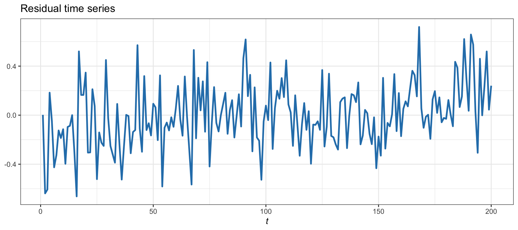
Figure 15.8: Cointegration residual for Example 15.1 with cointegration and low correlation.
| Test | \(p\)-value |
|---|---|
| ADF | 0.0081 |
| PP | 0.0001 |
| PGFF | 0.0001 |
| ERSD | 0.0008 |
| JOT | 0.0001 |
| SPR | 0.0001 |
Synthetic Data in Example 15.2
Consider now Example 15.2, and the corresponding Figure 15.5, where a synthetic non-cointegrated time series was generated with high correlation. The estimated cointegration relationship via least squares based on \(T=200\) observations is \[ \begin{aligned} y_{2t} &= 0.68 y_{1t} + 0.16 + r_t,\\ r_t &= 0.91 r_{t-1} + \epsilon_t, \end{aligned} \] where the residual \(r_t\) has a dangerous autoregressive coefficient of 0.91, which is close to 1, suggesting that the existence of a unit root cannot be excluded. This can be corroborated from the residual shown in Figure 15.9, with an estimated half-life of 7.29 (weak mean reversion). Additionally, Table 15.2 gives the \(p\)-values corresponding to several cointegration and residual unit-root tests. In this case, all the \(p\)-values are much higher than any reasonable threshold of, say, 0.01 and therefore the null hypothesis (existence of a unit root) cannot be rejected, which means we cannot conclude that the two time series are cointegrated.
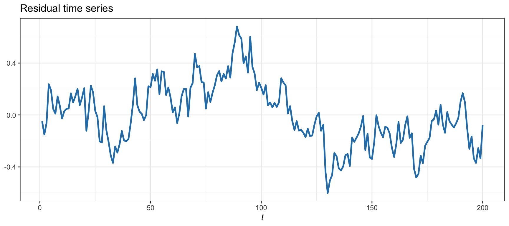
Figure 15.9: Cointegration residual for Example 15.2 with no cointegration and high correlation.
| Test | \(p\)-value |
|---|---|
| ADF | 0.4529 |
| PP | 0.0608 |
| PGFF | 0.0700 |
| ERSD | 0.0767 |
| JOT | 0.0996 |
| SPR | 0.2671 |
Market Data: EWA and EWC
EWA is an ETF that tracks the performance of the MSCI65 Australia Index, which includes Australian companies from various sectors such as financials, materials, healthcare, consumer staples, and energy. Similarly, EWC is an ETF that tracks the performance of the MSCI Canada Index. Thus, the EWA and EWC provide exposure to the Australian and Canadian equity markets, respectively, and can be used by investors to gain broad exposure to these countries’ economies.
EWA and EWC constitute a popular example in the quant community of cointegrated ETFs (Chan, 2013). The logic is that both the Canadian and Australian economies are commodity based, therefore their stock market performance is likely to be related through natural resources’ prices.
The cointegration relationship during 2016–2019 is estimated via least squares. When EWA is regressed against EWC, the resulting hedge ratio is \(\gamma=0.74\); but when EWC is regressed against EWA, we obtain 1.27, which is not exactly the inverse, \(1/0.74 \approx 1.35\). If instead we employ Johansen’s test, we obtain the more accurate weights of 1 for EWA and \(-0.80\) for EWC.
Figure 15.10 shows the residual of the cointegration relationship (spread), with an estimated half-life of 19 days (not very strong mean reversion). Table 15.3 shows the results for the cointegration tests, with the majority of the tests indicating cointegration at the 1% level (i.e., \(p\)-value less than 0.01), albeit two of the tests reject cointegration, so caution should be taken.
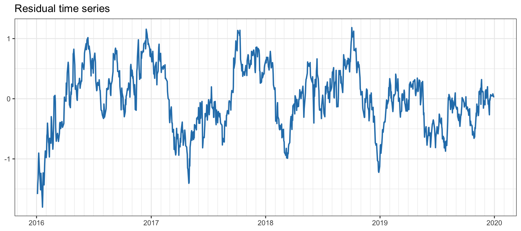
Figure 15.10: Cointegration residual for EWA–EWC.
| Test | \(p\)-value |
|---|---|
| ADF | 0.0049 |
| PP | 0.0058 |
| PGFF | 0.0062 |
| ERSD | 0.5310 |
| JOT | 0.0069 |
| SPR | 0.3840 |
Market Data: Coca-Cola and Pepsi
The stocks Coca-Cola (with ticker KO) and Pepsi (with ticker PEP) are often mentioned as an example of a pair of securities in the same industry group for which pairs trading might be fruitful. However, as already pointed out in Chan (2008), they do not seem to be cointegrated.
We assess the cointegration relationship during 2017–2019 via least squares. Their returns show a correlation of 0.66, which is statistically significant, but different from cointegration. Figure 15.11 shows the residual of the cointegration relationship (spread), with an estimated half-life of 70 days (not indicative of any cointegration). Table 15.4 shows the results for the cointegration tests, all of which reject the hypothesis of cointegration (all \(p\)-values are much larger than 0.01).
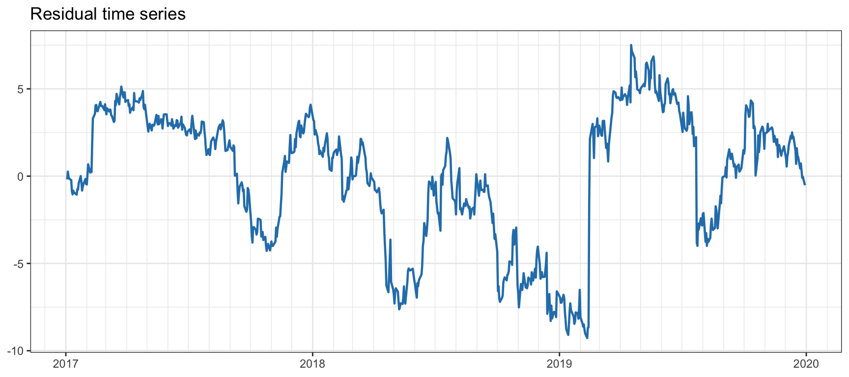
Figure 15.11: Cointegration residual for KO–PEP.
| Test | \(p\)-value |
|---|---|
| ADF | 0.2675 |
| PP | 0.1845 |
| PGFF | 0.1395 |
| ERSD | 0.0484 |
| JOT | 0.5627 |
| SPR | 0.1982 |
Market Data: SPY, IVV, and VOO
Standard & Poor’s 500 (S&P 500) is one of the world’s best-known indices and one of the most commonly used benchmarks for the U.S. stock market. There are a multitude of ETFs that track this index, such as Standard & Poor’s Depository Receipts SPY, iShares IVV, and Vanguard’s VOO. Given that they all track the same underlying asset, it is likely that these three ETFs will have a strong cointegrating relationship.
In this case, since we want to assess cointegration among more than two time series, namely, SPY, IVV, and VOO, we cannot use the Enger–Granger test. Instead, we have to resort to Johansen’s test, which first fits a VECM multivariate model and then proceeds to check sequentially the rank of matrix \(\bm{\Pi}\in\R^{3 \times 3}\), which satisfies \(0 \le r \le 3\).
Based on the period 2017–2019, Johansen’s test produces the following results:
- First, the null hypothesis is \(r=0\) vs. the alternative hypothesis \(r>0\): there is clear evidence to reject the null hypothesis.
- Then, the null hypothesis is \(r \le 1\) vs. the alternative hypothesis \(r>1\): again we have sufficient evidence to reject the null hypothesis.
- Finally, the null hypothesis is \(r \le 2\) vs. the alternative hypothesis \(r>2\): in this case we cannot reject the null hypothesis.
Thus, the conclusion is that the rank is \(r=2\), that is, we can find two different cointegrating relationships, whose residuals are shown in Figure 15.12.
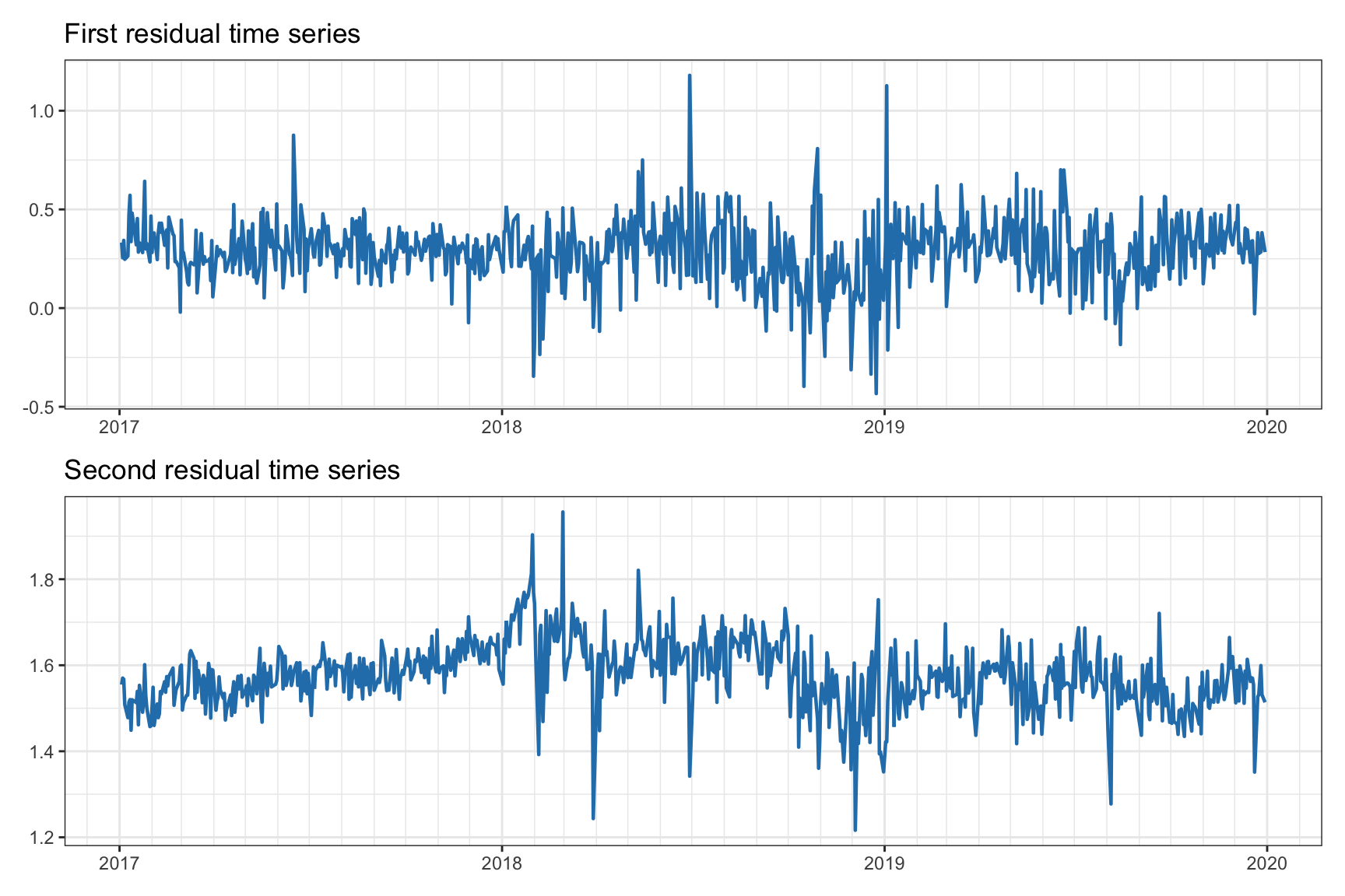
Figure 15.12: Cointegration residuals for SPY–IVV–VOO.
References
The Sveriges Riksbank Prize in Economic Sciences in Memory of Alfred Nobel 2003 was divided equally between Robert F. Engle III “for methods of analyzing economic time series with time-varying volatility (ARCH)” and Clive W. J. Granger “for methods of analyzing economic time series with common trends (cointegration).” ↩︎
The R packages
urcaandegcmimplement a long list of stationarity and cointegration tests (Clegg, 2023; Pfaff et al., 2022). ↩︎The \(p\)-value is the probability of obtaining the observed results under the assumption that the null hypothesis is correct. A small \(p\)-value means that there is strong evidence to reject the null hypothesis and accept the alternative hypothesis. Typical thresholds for determining whether a \(p\)-value is small enough are in the range 0.01–0.05.↩︎
Morgan Stanley Capital International (MSCI) is a leading provider of investment decision support tools and services. The company is best known for its global equity indices, which are widely used by investors to benchmark and analyze the performance of equity markets around the world.↩︎