11.5 Naive Diagonal Formulation
Consider the risk budgeting equations \[w_i\left(\bSigma\w\right)_i = b_i \, \w^\T\bSigma\w, \qquad i=1,\ldots,N.\] If we assume that the covariance matrix is diagonal, \(\bSigma = \textm{Diag}(\bm{\sigma}^2)\), then they simplify to \[w_i^2 \sigma_i^2 = b_i \sum_{j=1}^N w_j^2 \sigma_j^2, \qquad i=1,\ldots,N\] or, equivalently, \[\begin{equation} w_i = \frac{\sqrt{b_i}}{\sigma_i} \sqrt{\sum_{j=1}^N w_j^2 \sigma_j^2}, \qquad i=1,\ldots,N. \tag{11.2} \end{equation}\]
Observe that this portfolio is inversely proportional to the assets’ volatilities, which corresponds to the inverse volatility portfolio (IVolP) introduced in Section 6.5.2 of Chapter 6. Lower weights are given to high-volatility assets and higher weights to low-volatility assets, resulting in weighted constituent assets with equal volatility (for the case \(b_i=1/N\)): \[\textm{Std}(w_i x_i) = w_i\sigma_i = 1/N,\] where \(\textm{Std}(\cdot)\) denotes standard deviation.
For a general nondiagonal covariance matrix, a closed-form solution is not available and some optimization procedure has to be employed. Nevertheless, the diagonal solution in (11.2) can always be used as a “naive” solution. Interestingly, the diagonal solution is also optimal if the correlations of all assets are the same (Maillard et al., 2010).
11.5.1 Illustrative Example
Figure 11.2 shows the portfolio allocation and the risk contribution of the naive RPP and the \(1/N\) portfolio. The \(1/N\) portfolio has an equal capital allocation by definition, but it shows an unequal risk contribution with much more risk from the single-asset “MGM.” The naive RPP does a much better job equalizing the risk contribution, but it is not perfectly equalized since it ignores the off-diagonal elements of the covariance matrix.
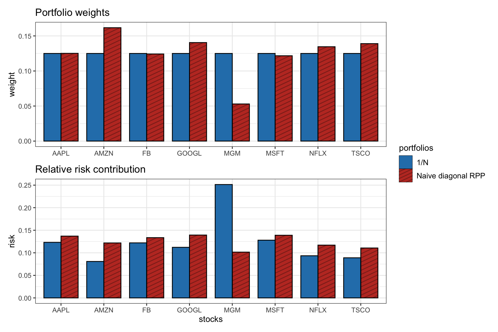
Figure 11.2: Portfolio allocation and risk contribution of the \(1/N\) portfolio and naive diagonal RPP.