9.4 Algorithms
We will focus only on the MVSK portfolio formulation (9.11), whose objective function, \[\begin{equation} f(\w) = - \lambda_1 \phi_1(\w) + \lambda_2 \phi_2(\w) - \lambda_3 \phi_3(\w) + \lambda_4 \phi_4(\w), \tag{9.15} \end{equation}\] is nonconvex due to the higher-order moments.
It is convenient to split the nonconvex MVSK objective function (9.15) into convex and nonconvex terms: \[f(\w) = f_\textm{cvx}(\w) + f_\textm{ncvx}(\w),\] where \[ \begin{aligned} f_\textm{cvx}(\w) & = - \lambda_1 \phi_1(\w) + \lambda_2 \phi_2(\w),\\ f_\textm{ncvx}(\w) & = - \lambda_3 \phi_3(\w) + \lambda_4 \phi_4(\w). \end{aligned} \]
One can, of course, always use some off-the-shelf general nonconvex solver (typically referred to as a nonlinear solver) capable of dealing with the nonconvex MVSK portfolio formulation (9.11). In the following, however, we will develop ad hoc methods that are much more efficient and do not require the use of a general nonlinear solver. In particular, we will explore the successive convex approximation (SCA) framework as well as the majorization–minimization (MM) framework for the derivation of the numerical methods (see Appendix B for details on numerical methods).
9.4.1 Via the SCA Framework
Preliminaries on SCA
The successive convex approximation method (or framework) approximates a difficult optimization problem by a sequence of simpler convex approximated problems. For details, the reader is referred to Section B.8 in Appendix B, the original paper in Scutari et al. (2014), and the comprehensive book chapter in Scutari and Sun (2018). We now give a concise description.
Suppose the following (difficult) problem is to be solved: \[ \begin{array}{ll} \underset{\bm{x}}{\textm{minimize}} & f(\bm{x})\\ \textm{subject to} & \bm{x} \in \mathcal{X}, \end{array} \] where \(f(\cdot)\) is the (possibly nonconvex) objective function and \(\mathcal{X}\) is a convex set. Instead of attempting to directly obtain a solution \(\bm{x}^\star\) (either a local or global solution), the SCA method will produce a sequence of iterates \(\bm{x}^0, \bm{x}^1, \bm{x}^2,\dots\) that will converge to \(\bm{x}^\star\).
More specifically, at iteration \(k\), the SCA approximates the objective function \(f(\bm{x})\) by a surrogate function around the current point \(\bm{x}^k\), denoted by \(\tilde{f}\left(\bm{x};\bm{x}^k\right)\). One may be tempted to solve the sequence of (simpler) problems \[ \bm{x}^{k+1}=\underset{\bm{x}\in\mathcal{X}}{\textm{arg min}}\;\tilde{f}\left(\bm{x};\bm{x}^k\right), \qquad k=0,1,2,\dots \]
Unfortunately, the previous sequence of updates may not converge and a smoothing step is necessary to introduce some memory in the process, which will avoid undesired oscillations. Thus, the correct sequence of problems in the SCA method is \[ \begin{array}{ll} \left. \begin{aligned} \hat{\bm{x}}^{k+1} &= \underset{\bm{x}\in\mathcal{X}}{\textm{arg min}}\;\tilde{f}\left(\bm{x};\bm{x}^k\right)\\ \bm{x}^{k+1} &= \bm{x}^{k} + \gamma^k \left(\hat{\bm{x}}^{k+1} - \bm{x}^{k}\right) \end{aligned} \quad \right\} \qquad k=0,1,2,\dots, \end{array} \] where \(\{\gamma^k\}\) is a properly designed sequence with \(\gamma^k \in (0,1]\) (Scutari et al., 2014).
In order to guarantee converge of the iterates, the surrogate function \(\tilde{f}\left(\bm{x};\bm{x}^k\right)\) has to satisfy the following technical conditions (Scutari et al., 2014):
- \(\tilde{f}\left(\bm{x};\bm{x}^k\right)\) must be strongly convex on the feasible set \(\mathcal{X}\); and
- \(\tilde{f}\left(\bm{x};\bm{x}^k\right)\) must be differentiable with \(\nabla\tilde{f}\left(\bm{x};\bm{x}^k\right) = \nabla f\left(\bm{x}\right)\).
SCA Applied to MVSK Portfolio Design
Following the SCA framework, we will leave \(f_\textm{cvx}(\w)\) untouched, since it is already (strongly) convex, and we will construct a quadratic convex approximation (another option would be a linear approximation) of the nonconvex term \(f_\textm{ncvx}(\w)\) around the point \(\w=\w^k\) as \[ \begin{aligned} \tilde{f}_\textm{ncvx}\left(\w; \w^k\right) &= f_\textm{ncvx}\left(\w^k\right) + \nabla f_\textm{ncvx}\left(\w^k\right)^\T \left(\w - \w^k\right)\\ & \quad + \frac{1}{2} \left(\w - \w^k\right)^\T \left[\nabla^2 f_\textm{ncvx}\left(\w^k\right)\right]_\textm{PSD} \left(\w - \w^k\right), \end{aligned} \] where \(\left[\bm{\Xi}\right]_\textm{PSD}\) denotes the projection of the matrix \(\bm{\Xi}\) onto the set of positive semidefinite matrices. In practice, this projection can be obtained by first computing the eigenvalue decomposition of the matrix, \(\bm{\Xi} = \bm{U}\textm{Diag}\left(\bm{\lambda}\right)\bm{U}^\T\), and then projecting the eigenvalues onto the nonnegative orthant \(\left[\bm{\Xi}\right]_\textm{PSD} = \bm{U}\textm{Diag}\left(\bm{\lambda}^+\right)\bm{U}^\T,\) where \((\cdot)^+=\textm{max}(0,\cdot).\) [As a technical detail, if \(\lambda_2=0\), then the matrix \(\left[\bm{\Xi}\right]_\textm{PSD}\) should be made positive definite so that the overall approximation is strongly convex (Zhou and Palomar, 2021).]
Thus, a quadratic convex approximation of \(f(\w)\) in (9.15) is obtained as \[ \begin{aligned} \tilde{f}\left(\w; \w^k\right) &= f_\textm{cvx}(\w) + \tilde{f}_\textm{ncvx}\left(\w; \w^k\right)\\ &= \frac{1}{2}\w^\T\bm{Q}^k\w + \w^\T\bm{q}^k + \textm{constant}, \end{aligned} \] where \[ \begin{aligned} \bm{Q}^k &= \lambda_2 \nabla^2\phi_2(\w) + \left[\nabla^2 f_\textm{ncvx}\left(\w^k\right)\right]_\textm{PSD},\\ \bm{q}^k &= - \lambda_1 \nabla\phi_1(\w) + \nabla f_\textm{ncvx}\left(\w^k\right) - \left[\nabla^2 f_\textm{ncvx}\left(\w^k\right)\right]_\textm{PSD}\w^k, \end{aligned} \] and the gradients and Hessians of the moments can be obtained from either the nonparametric expressions in (9.2)–(9.3) or the parametric ones in (9.7)–(9.8).
Finally, the SCA-based algorithm can be implemented by successively solving, for \(k=0,1,2,\dots\), the convex quadratic problems \[\begin{equation} \begin{array}{ll} \underset{\w}{\textm{minimize}} & \frac{1}{2}\w^\T \bm{Q}^k\w + \w^\T\bm{q}^k\\ \textm{subject to} & \w \in \mathcal{W}. \end{array} \tag{9.16} \end{equation}\]
This SCA-based quadratic approximated MVSK (SCA-Q-MVSK) method is summarized in Algorithm 9.1. More details and similar algorithms for other formulations, such as MVSK portfolio tilting, can be found in Zhou and Palomar (2021).
Algorithm 9.1: SCA-Q-MVSK method to solve the MVSK portfolio in (9.11).
Choose initial point \(\w^0\in\mathcal{W}\) and sequence \(\{\gamma^k\}\);
Set \(k \gets 0\);
repeat
- Calculate \(\nabla f_\textm{ncvx}\left(\w^k\right)\) and \(\left[\nabla^2 f_\textm{ncvx}\left(\w^k\right)\right]_\textm{PSD}\);
- Solve the problem (9.16) and keep solution as \(\hat{\w}^{k+1}\);
- \(\w^{k+1} \gets \w^{k} + \gamma^k (\hat{\w}^{k+1} - \w^{k})\);
- \(k \gets k+1\);
until convergence;
9.4.2 Via the MM Framework
Preliminaries on MM
The majorization–minimization method (or framework), similarly to SCA, approximates a difficult optimization problem by a sequence of simpler approximated problems. We now give a concise description. For details, the reader is referred to Section B.7 in Appendix B, as well as the concise tutorial in Hunter and Lange (2004), the long tutorial with applications in Y. Sun et al. (2017), and the convergence analysis in Razaviyayn et al. (2013).
Suppose the following (difficult) problem is to be solved: \[ \begin{array}{ll} \underset{\bm{x}}{\textm{minimize}} & f(\bm{x})\\ \textm{subject to} & \bm{x} \in \mathcal{X}, \end{array} \] where \(f(\cdot)\) is the (possibly nonconvex) objective function and \(\mathcal{X}\) is a (possibly nonconvex) set. Instead of attempting to directly obtain a solution \(\bm{x}^\star\) (either a local or global solution), the MM method will produce a sequence of iterates \(\bm{x}^0, \bm{x}^1, \bm{x}^2,\dots\) that will converge to \(\bm{x}^\star\).
More specifically, at iteration \(k\), the MM approximates the objective function \(f(\bm{x})\) by a surrogate function around the current point \(\bm{x}^k\) (essentially, a tangent upper bound), denoted by \(u\left(\bm{x};\bm{x}^k\right)\), leading to the sequence of (simpler) problems \[ \bm{x}^{k+1}=\underset{\bm{x}\in\mathcal{X}}{\textm{arg min}}\;u\left(\bm{x};\bm{x}^k\right), \qquad k=0,1,2,\dots \]
In order to guarantee convergence of the iterates, the surrogate function \(u\left(\bm{x};\bm{x}^k\right)\) has to satisfy the following technical conditions (Razaviyayn et al., 2013; Y. Sun et al., 2017):
- upper bound property: \(u\left(\bm{x};\bm{x}^k\right) \geq f\left(\bm{x}\right)\);
- touching property: \(u\left(\bm{x}^k;\bm{x}^k\right) = f\left(\bm{x}^k\right)\); and
- tangent property: \(u\left(\bm{x};\bm{x}^k\right)\) must be differentiable with \(\nabla u\left(\bm{x};\bm{x}^k\right) = \nabla f\left(\bm{x}\right)\).
The surrogate function \(u\left(\bm{x};\bm{x}^k\right)\) is also referred to as the majorizer because it is an upper bound of the original function. The fact that, at each iteration, first the majorizer is constructed and then it is minimized gives the name majorization–minimization to the method.
MM Applied to MVSK Portfolio Design
Following the MM framework, we will leave \(f_\textm{cvx}(\w)\) untouched, since it is already convex, and we will construct a majorizer (i.e., a tangent upper-bound surrogate function) of the nonconvex term \(f_\textm{ncvx}(\w)\) around the point \(\w=\w^k\). For example, a linear function plus a quadratic regularizer, \[ \tilde{f}_\textm{ncvx}\left(\w; \w^k\right) = f_\textm{ncvx}\left(\w^k\right) + \nabla f_\textm{ncvx}\left(\w^k\right)^\T \left(\w - \w^k\right) + \frac{\tau_\textm{MM}}{2} \|\w - \w^k\|_2^2, \] where \(\tau_\textm{MM}\) is a positive constant properly chosen so that \(\tilde{f}_\textm{ncvx}\left(\w; \w^k\right)\) upper-bounds \(f_\textm{ncvx}(\w)\) (Zhou and Palomar, 2021).
Thus, a quadratic convex approximation of \(f(\w)\) (albeit using only first-order or linear information about the nonconvex term \(f_\textm{ncvx}\)) is obtained as \[ \begin{aligned} \tilde{f}\left(\w; \w^k\right) &= f_\textm{cvx}(\w) + \tilde{f}_\textm{ncvx}\left(\w; \w^k\right)\\ &= - \lambda_1 \phi_1(\w) + \lambda_2 \phi_2(\w) + \nabla f_\textm{ncvx}\left(\w^k\right)^\T \w + \frac{\tau_\textm{MM}}{2} \|\w - \w^k\|_2^2 + \textm{constant}, \end{aligned} \] where the gradient of the nonconvex function \(f_\textm{ncvx}\) can be obtained from the gradients of \(\phi_3(\w)\) and \(\phi_4(\w)\), either the nonparametric expressions in (9.2) or the parametric ones in (9.7). It is worth pointing out that, owing to the linear approximation of the nonconvex term \(f_\textm{ncvx}(\w)\), the Hessians are not even required, which translates into huge savings in computation time and storage memory.
Finally, the MM-based algorithm can be implemented by successively solving, for \(k=0,1,2,\dots\), the convex problems \[\begin{equation} \begin{array}{ll} \underset{\w}{\textm{minimize}} & - \lambda_1 \phi_1(\w) + \lambda_2 \phi_2(\w)+ \nabla f_\textm{ncvx}\left(\w^k\right)^\T \w + \frac{\tau_\textm{MM}}{2} \|\w - \w^k\|_2^2\\ \textm{subject to} & \w \in \mathcal{W}. \end{array} \tag{9.17} \end{equation}\] We denote the solution to each majorized problem in (9.17) as \(\textm{MM}(\w^k)\), so that \(\w^{k+1} = \textm{MM}(\w^k)\).
Unfortunately, due to the upper-bound requirement of the nonconvex function \(\tilde{f}_\textm{ncvx}\left(\w; \w^k\right)\), the constant \(\tau_\textm{MM}\) ends up being too large in practice. This means that the approximation is not tight enough and the method requires many iterations to converge. For that reason, it is necessary to resort to some acceleration techniques.
We consider a quasi-Newton acceleration technique called SQUAREM (Varadhan and Roland, 2008) that works well in practice. Instead of taking the solution to the majorized problem in (9.17), \(\textm{MM}(\w^k)\), as the next point \(\w^{k+1}\), the acceleration technique takes two steps and combines them in a sophisticated way, with a final third step to guarantee feasibility. The details are as follows: \[\begin{equation} \begin{aligned} \textm{difference first update:} \qquad \bm{r}^k &= R(\w^k) = \textm{MM}(\w^k) - \w^k\\ \textm{difference of differences:} \qquad \bm{v}^k &= R(\textm{MM}(\w^k)) - R(\w^k)\\ \textm{stepsize:} \qquad \alpha^k &= -\textm{max}\left(1, \|\bm{r}^k\|_2/\|\bm{v}^k\|_2\right)\\ \textm{actual step taken:} \qquad \bm{y}^k &= \w^k - \alpha^k \bm{r}^k\\ \textm{final update on actual step:} \quad \bm{w}^{k+1} &= \textm{MM}(\bm{y}^k). \end{aligned} \tag{9.18} \end{equation}\] The choice of the stepsize \(\alpha^k\) can be further refined to get a more robust algorithm with a much faster convergence (X. Wang et al., 2023). The last step, \(\bm{w}^{k+1}=\textm{MM}(\bm{y}^k)\), can also be simplified to avoid having to solve the majorized problem a third time.
This quasi-Newton accelerated MM linear (as in using linear information or gradient only of the nonconvex term) MVSK (Acc-MM-L-MVSK) method is summarized in Algorithm 9.2. More details and similar algorithms for other formulations, such as MVSK portfolio tilting, can be found in X. Wang et al. (2023).47
Algorithm 9.2: Acc-MM-L-MVSK method to solve the MVSK portfolio in (9.11).
Choose initial point \(\w^0\in\mathcal{W}\) and proper constant \(\tau_\textm{MM}\) for majorized problem (9.17);
Set \(k \gets 0\);
repeat
- Calculate \(\nabla f_\textm{ncvx}\left(\w^k\right)\);
- Compute the quantities \(\bm{r}^k,\) \(\bm{v}^k,\) \(\alpha^k,\) \(\bm{y}^k,\) and current solution \(\bm{w}^{k+1}\) as in (9.18), which requires solving the majorized problem (9.17) three times;
- \(k \gets k+1\);
until convergence;
9.4.3 Numerical Experiments
We now perform an empirical study and comparison of the computational cost of the two methods SCA-Q-MVSK and Acc-MM-L-MVSK described in Algorithms 9.1 and 9.2, respectively. In addition, for the computation of the gradients and Hessians of the moments, we consider both the nonparametric expressions in (9.2)–(9.3) and the parametric ones in (9.7)–(9.8).
In fact, the Acc-MM-L-MVSK method considered in the numerical results is actually an improvement over Algorithm 9.2 that does not require the computation of the constant \(\tau_\textm{MM}\) in (9.17) (which already takes on the order of 10 seconds for \(N=100\)). For details refer to X. Wang et al. (2023).
Convergence and Computation Time
Figure 9.4 shows the convergence of different MVSK portfolio optimization methods for a universe size of \(N=100\). In this case, both the nonparametric and parametric expressions for the moments can be employed. As a reference, the benchmark computation of the solution via an off-the-shelf nonlinear solver requires around 5 seconds with nonparametric moments and around 0.5 seconds with parametric moments.
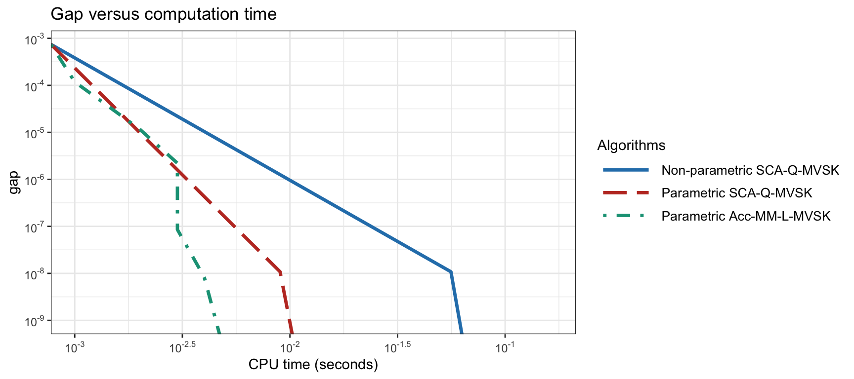
Figure 9.4: Convergence of different MVSK portfolio optimization algorithms for \(N=100\).
Figure 9.5 similarly shows the convergence of different MVSK portfolio optimization methods for a universe size of \(N=400\). In this case, however, due to the larger universe size, only the parametric computation of the moments is feasible. As a reference, the benchmark computation of the solution via an off-the-shelf nonlinear solver requires around 1 minute.
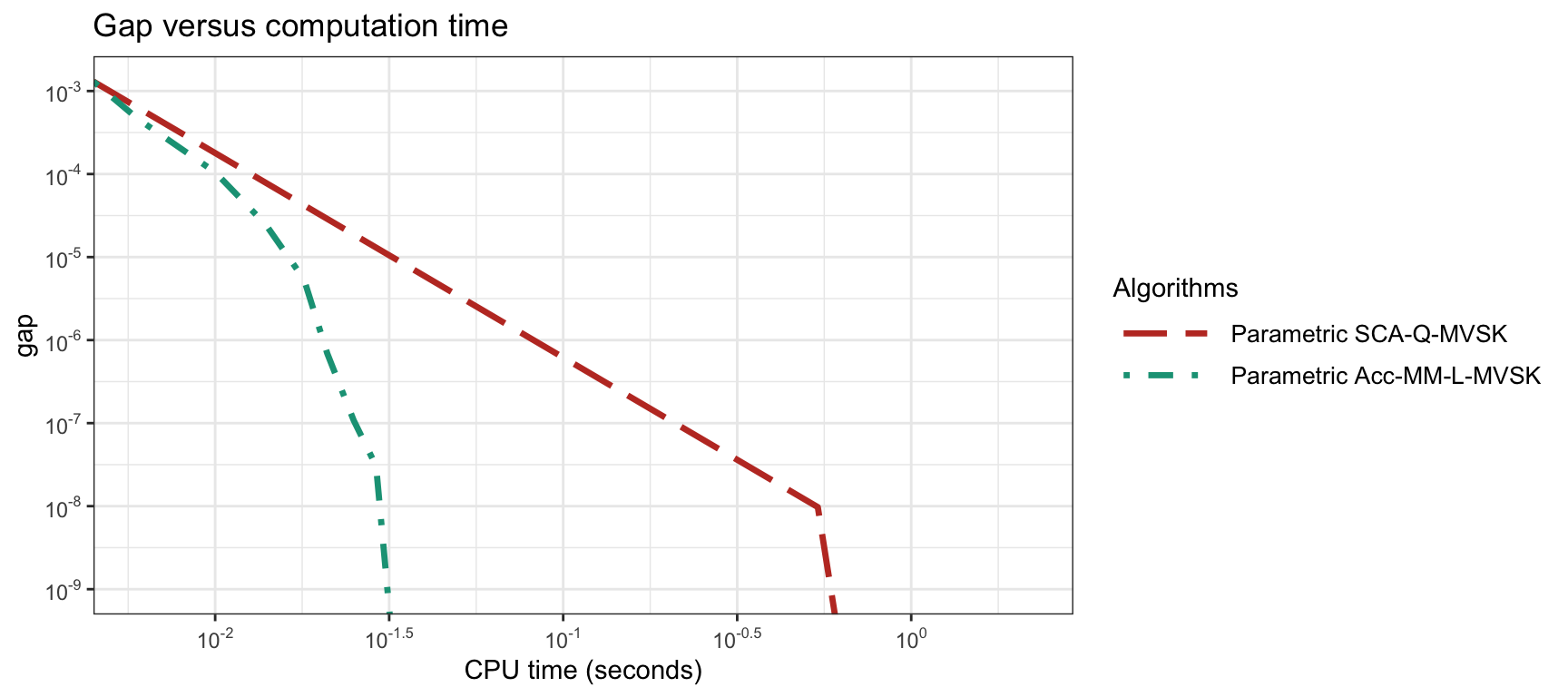
Figure 9.5: Convergence of different MVSK portfolio optimization algorithms for \(N=400\).
Figure 9.6 shows a boxplot of the computation time vs. the universe dimension \(N\) for different MVSK portfolio optimization methods (in the parametric case).
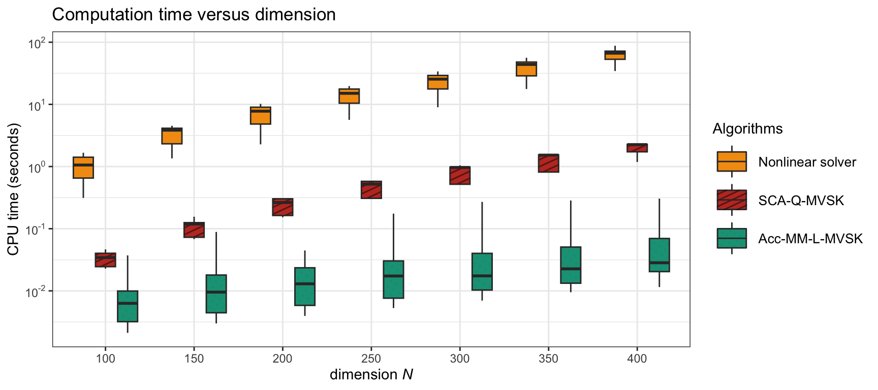
Figure 9.6: Computation time of different (parametric) MVSK portfolio optimization algorithms.
More extensive numerical comparisons can be found in Zhou and Palomar (2021) and X. Wang et al. (2023).
Summarizing, it seems clear that parametric computation of the moments is the most appropriate (due to the otherwise high computational cost). In addition, the Acc-MM-L-MVSK method described in Algorithm 9.2 – to be exact, the more sophisticated version proposed in X. Wang et al. (2023)) – provides the fastest convergence by orders of magnitude.
Portfolio Backtest
We compare the performance of some portfolios based on different moments, namely, the global maximum return portfolio (GMRP; see Section 6.4.2 in Chapter 6), the global minimum variance portfolio (GMVP; see Section 6.5.1 in Chapter 6), and the MVSK portfolio in (9.11) (setting \(\lambda_1=0\) to resemble the GMVP).
Figure 9.7 shows the cumulative P&L and drawdown during 2016–2019 over a random universe of 20 stocks from the S&P 500, whereas Table 9.1 gives the numerical values over the whole period. A small improvement of the MVSK portfolio over the GMVP can be observed.
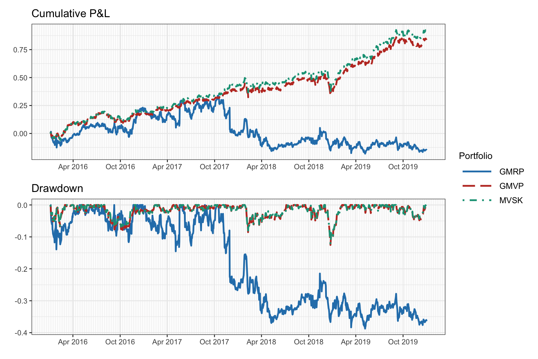
Figure 9.7: Backtest of high-order portfolios: cumulative P&L and drawdown.
| Portfolio | Sharpe ratio | Annual return | Annual volatility | Sortino ratio | Max drawdown | CVaR (0.95) |
|---|---|---|---|---|---|---|
| GMRP | \(-0.01\) | 0% | 27% | \(-0.02\) | 39% | 4% |
| GMVP | \(1.47\) | 16% | 11% | \(2.12\) | 13% | 2% |
| MVSK | \(1.56\) | 17% | 11% | \(2.26\) | 12% | 2% |
Multiple Portfolio Backtests
We now consider multiple randomized backtests (see Section 8.4 in Chapter 8) for a better characterization of the performance of the portfolios. We take a dataset of \(N=20\) stocks over the period 2015–2020 and generate 100 resamples each with \(N=8\) randomly selected stocks and a random period of two years. Then we perform a walk-forward backtest with a lookback window of 1 year, reoptimizing the portfolio every month.
Figure 9.8 shows the boxplots of the Sharpe ratio and maximum drawdown, and Table 9.2 shows the backtest results in table form with different performance measures over the whole period. Again, one can observe a modest improvement of the MVSK portfolio over the GMVP.
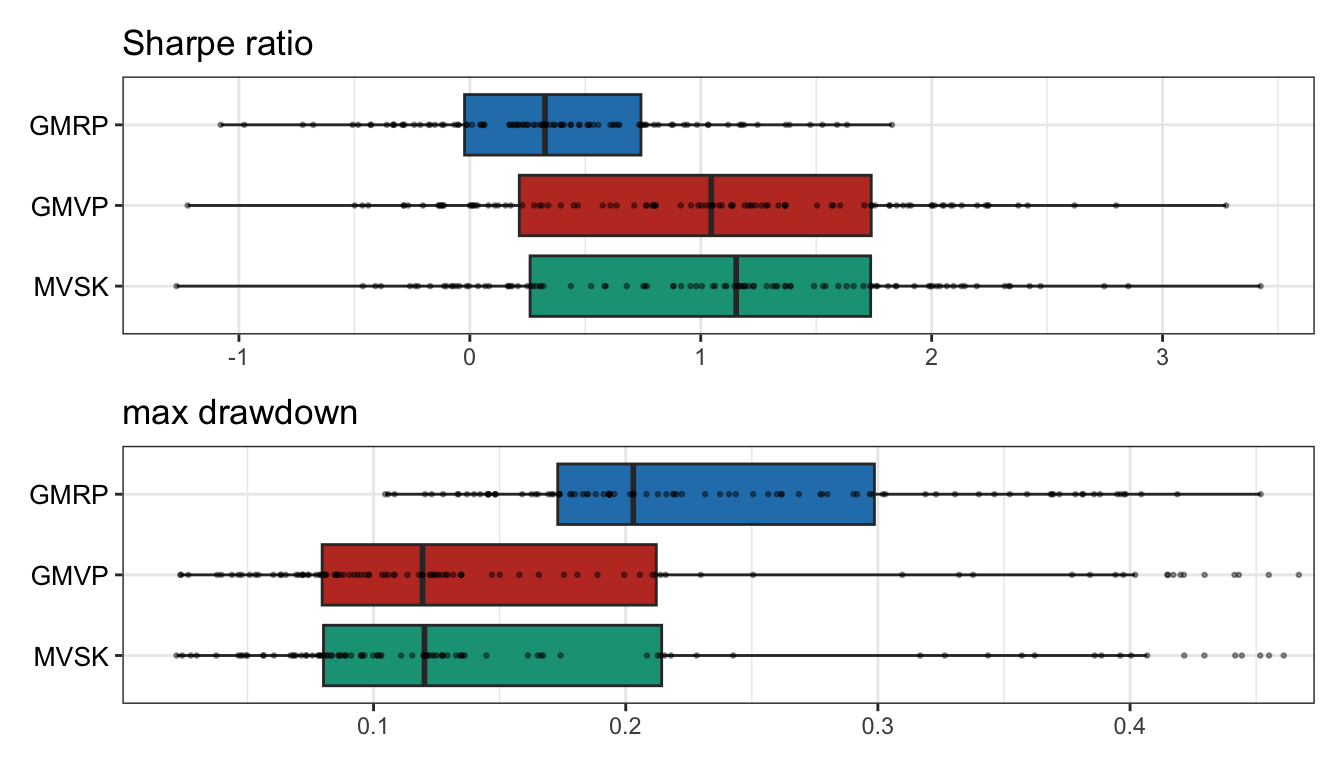
Figure 9.8: Multiple randomized backtest of high-order portfolios: Sharpe ratio and maximum drawdown.
| Portfolio | Sharpe ratio | Annual return | Annual volatility | Sortino ratio | Max drawdown | CVaR (0.95) |
|---|---|---|---|---|---|---|
| GMRP | 0.33 | 9% | 26% | 0.45 | 20% | 4% |
| GMVP | 1.05 | 13% | 13% | 1.48 | 12% | 2% |
| MVSK | 1.15 | 14% | 13% | 1.58 | 12% | 2% |
References
The R package
highOrderPortfolios(Zhou, Wang, et al., 2022) implements Algorithms 9.1 and 9.2 based on Zhou and Palomar (2021) and X. Wang et al. (2023). ↩︎