8.5 Backtesting with Synthetic Data
As we have already discussed, a backtest evaluates the out-of-sample performance of an investment strategy using past observations. Section 8.4 has explored different ways to directly use the historical data to assess the performance as if the strategy had been run in the past. This section considers a more indirect way to employ historical data by generating synthetic – yet realistic – data to simulate scenarios that did not happen in the past, such as stress tests where different market scenarios are recreated to test the strategy.
Monte Carlo simulations allow us to create synthetic data that resembles a given set of historical data. They can be divided into three categories:
- Parametric methods: These postulate and fit a model to the data. Then, they generate as much synthetic data as necessary from the model.
- Nonparametric methods: These directly resample the historical data without any modeling.
- Hybrid methods: These combine the modeling approach with resampling for the model residual (which can follow a parametric or nonparametric method).
Generating such realistic synthetic data will allow us to backtest a strategy on a large number of unseen, synthetic testing sets, hence reducing the likelihood that the strategy has been fitted to a particular dataset. The quality of the data generated under parametric methods depends on the model assumption: if the model is wrong, the data generated will not be realistic. Nonparametric methods are more robust, but they can also potentially destroy some temporal structure in the data. Hybrid methods are more appealing as they can model as much structure as possible and then the residual data is that generated following either the parametric or nonparametric approach. These methods are compared and illustrated next.
8.5.1 I.I.D. Assumption
The simplest possible example of a parametric method is based on modeling the returns as i.i.d. and fitting some distribution function, such as Gaussian or preferably a heavy-tailed distribution. Once the parameters of the distribution have been estimated (i.e., the model has been fitted to the data), then synthetic data can be generated, which will resemble (statistically) the original data.
The simplest example of a nonparametric method, also based on assuming the returns are i.i.d., is even simpler to implement: just resample the original returns with replacement.
It is important to emphasize that these two examples of parametric and nonparametric methods are based on the i.i.d. assumption, which obviously does not hold for financial data (e.g., the absolute values of the returns are highly correlated as observed in Chapter 2, Figures 2.19–2.22).
Figure 8.17 illustrates the synthetic generation of return data under the i.i.d. parametric (assuming a Gaussian distribution) and nonparametric methods. Since both methods assume i.i.d. data, they totally destroy the volatility clustering structure present in the original data. In addition, the parametric method is assuming (wrongly) a Gaussian distribution and therefore the generated data does not have the same deep spikes typical of a heavy-tailed distribution. The nonparametric method, on the other hand, includes deep spikes but dispersed over time rather than clustered. We next consider a more realistic case by incorporating the temporal structure.
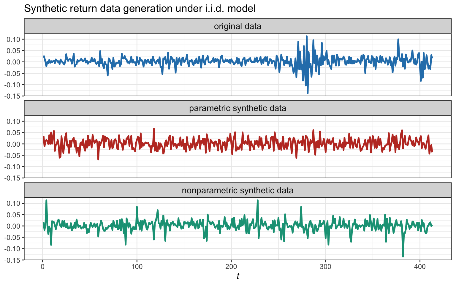
Figure 8.17: Example of an original sequence and two synthetic sequences generated with i.i.d. parametric and nonparametric methods.
8.5.2 Temporal Structure
To illustrate the hybrid method, suppose now that a more sophisticated model is used to model the expected returns based on the past values of the returns, denoted by \(\bmu_t = \bm{f}(\bm{r}_{t-k},\dots,\bm{r}_{t-1})\) (see Chapter 4 for time-series mean models). This means that the returns can be written as the forecast plus some residual error, \[ \bm{r}_{t} = \bmu_t + \bm{u}_t, \] where \(\bm{u}_t\) is the zero-mean residual error at time \(t\) with covariance matrix \(\bSigma\).
An even more sophisticated model can combine the mean model for \(\bmu_t\) with a covariance model for \(\bSigma_t\): \[ \bm{r}_{t} = \bmu_t + \bSigma_t^{1/2}\bm{\epsilon}_t, \] where \(\bm{\epsilon}_t\) is a standardized zero-mean identity-covariance residual error at time \(t\). The reader is referred to Chapter 4 for time-series mean and covariance models.
In these more sophisticated modeling cases, we can now take two different approaches to generate the sequence of residuals and, implicitly, the sequence of synthetic returns:
- following the parametric paradigm: we can model the residuals with an i.i.d. model and generate new synthetic residuals; and
- following the nonparametric paradigm: we can just resample the residuals from the historical data.
Figure 8.18 illustrates the synthetic generation of return data properly modeling the volatility clustering and then using both the parametric (assuming a Gaussian distribution) and nonparametric methods. As expected, the volatility clustering is preserved as it appears in the original data. The parametric method is assuming (wrongly) a Gaussian distribution for the residuals and it could be further improved by employing a heavy-tailed distribution. The nonparametric method, on the other hand, is more robust to modeling errors since it is directly resampling the original residuals.
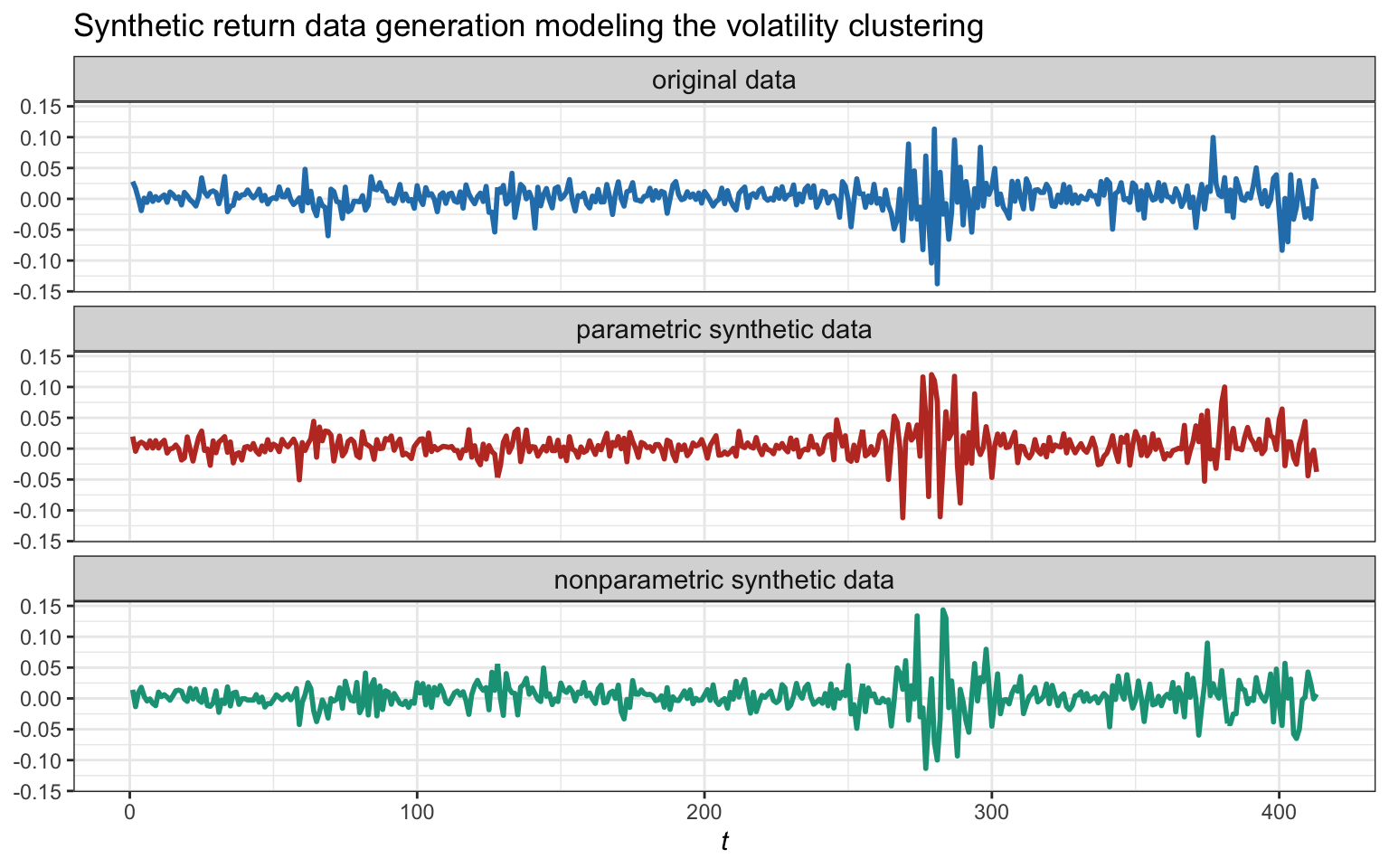
Figure 8.18: Example of an original sequence and two synthetic sequences generated by modeling the volatility clustering and the residuals with parametric and nonparametric methods.
8.5.3 Stress Tests
Stress tests are yet another set of tools in the backtest toolkit. They also fall into the category of synthetic generated data but they are more like an “à la carte menu.” The idea is to be able to generate realistic synthetic data recreating different market scenarios, such as the choice of a strong bull market, a weak bull market, a side market, a weak bear market, and a strong bear market.
Other examples of stress tests could consider specific periods of crises such as the stock market crash of October 1987, the Asian crisis of 1997, and the tech bubble that burst in 1999–2000.
In other words, stress testing tests the resilience of investment portfolios against possible future financial situations.
Figure 8.19 illustrates the generation of synthetic data for stress testing corresponding to a bull market (the reference bull market period is April–August, 2020). On the other hand, Figure 8.20 illustrates the generation of synthetic data for stress testing corresponding to a bear market (the reference bear market period is September–December, 2018).
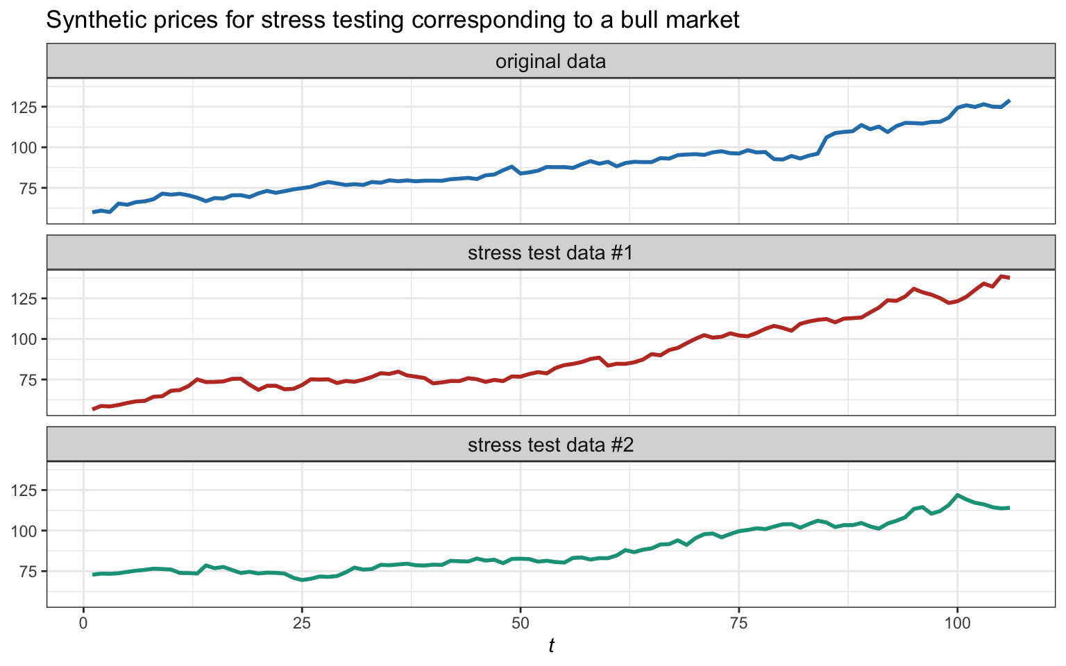
Figure 8.19: Example of original data corresponding to a bull market and two synthetic generations of bull markets for stress testing.
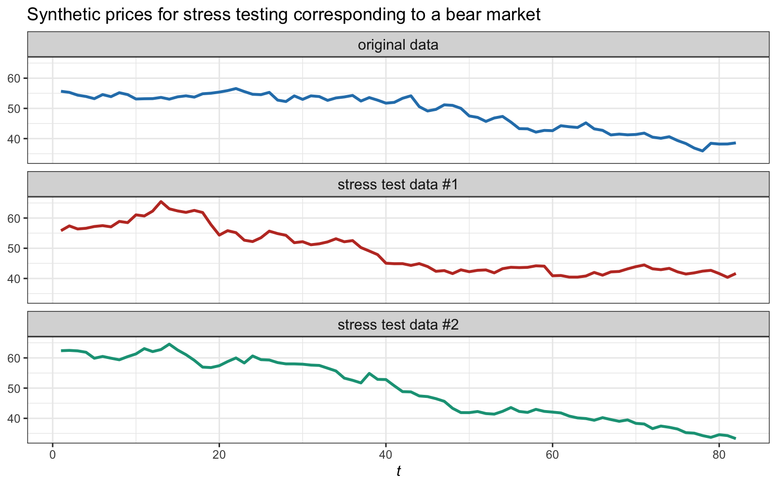
Figure 8.20: Example of original data corresponding to a bear market and two synthetic generations of bear markets for stress testing.