3.3 Location Estimators
From the i.i.d. model in (3.1), the parameter \(\bmu\) can be interpreted as the “center” or “location” around which the random points are distributed. Thus, it makes sense to try to estimate this location, which can be done in a variety of ways. The classical approach is based on least squares fitting, but it is very sensitive to extreme observations and missing values; thus, alternative robust multivariate location estimators have been thoroughly studied in the literature. In fact, this topic can be traced back to the 1960s (Huber, 1964; Maronna, 1976), as surveyed in Small (1990), Huber (2011), and Oja (2013).
3.3.1 Least Squares Estimator
The method of least squares (LS) dates back to 1795 when Gauss used it to study planetary motions. It deals with the linear model \(\bm{y} = \bm{A}\bm{x} + \bm{\epsilon}\) by solving the problem (Kay, 1993; Scharf, 1991) \[ \begin{array}{ll} \underset{\bm{x}}{\textm{minimize}} & \left\Vert \bm{y} - \bm{A}\bm{x} \right\Vert_2^2, \end{array} \] which has the closed-form solution \(\bm{x}^{\star}=\left(\bm{A}^\T\bm{A}\right)^{-1}\bm{A}^\T\bm{y}\).
Going back to the i.i.d. model in (3.1), we can now formulate the estimation of the center of the points, \(\bm{x}_t = \bmu + \bm{\epsilon}_t\), as an LS problem: \[ \begin{array}{ll} \underset{\bmu}{\textm{minimize}} & \begin{aligned}[t] \sum_{t=1}^{T} \left\Vert \bm{x}_t - \bmu \right\Vert_2^2 \end{aligned}, \end{array} \] whose solution, interestingly, coincides with the sample mean in (3.2): \[ \hat{\bmu} = \frac{1}{T}\sum_{t=1}^{T}\bm{x}_{t}. \]
The sample mean is well known to suffer from lack of robustness against contaminated points or outliers, as well as against distributions with heavy tails (as will be empirically verified later in Figure 3.4).
3.3.2 Median Estimator
The median of a sample of points is the value separating the higher half from the lower half of the points. It may be thought of as the “middle” value of the points. The main advantage of the median compared to the mean (often described as the “average”) is that it is not affected by a small proportion of extremely large or small values. Thus, it is a natural robust estimate and provides a better representation of a “typical” value. It is also possible to further improve on the median by using additional information from the data points such as the sample size, range, and quartile values (Wan et al., 2014).
In the multivariate case, there are multiple ways to extend the concept of median, as surveyed in Small (1990), Huber (2011), and Oja (2013), to obtain a natural robust estimate of the center of the distribution or set of points. One straightforward extension consists of employing the univariate median elementwise.
In the context of the i.i.d. model in (3.1), it turns out that this elementwise median can be formulated as the solution to the following problem: \[\begin{array}{ll} \underset{\bmu}{\textm{minimize}} & \begin{aligned}[t] \sum_{t=1}^{T} \left\Vert \bm{x}_t - \bmu \right\Vert_1 \end{aligned}, \end{array} \] where now the \(\ell_1\)-norm is the measure of error instead of the squared \(\ell_2\)-norm as in the case of the sample mean.
3.3.3 Spatial Median Estimator
Another way to extend the univariate median to the multivariate case is the so-called spatial median or geometric median (also known as the \(L_1\) median) obtained as the solution to the problem \[ \begin{array}{ll} \underset{\bmu}{\textm{minimize}} & \begin{aligned}[t] \sum_{t=1}^{T} \left\Vert \bm{x}_t - \bmu \right\Vert_2 \end{aligned}, \end{array} \] where now the \(\ell_2\)-norm or Euclidean distance is the measure of error instead of the \(\ell_1\)-norm or the squared \(\ell_2\)-norm. Interestingly, the lack of the squaring operator has a huge effect; for example, the estimator for each element is no longer independent of the other elements (as is the case with the sample mean and elementwise median). The spatial median has the desired property that for \(N=1\) it reduces to the univariate median.
The spatial median is the solution to a convex second-order cone problem (SOCP) and can be solved with an SOCP solver. Alternatively, very efficient iterative algorithms can be derived by solving a sequence of LS problems via the majorization–minimization (MM) method (Y. Sun et al., 2017); see also Section B.7 in Appendix B for details.
3.3.4 Numerical Experiments
Figure 3.3 illustrates the different location estimators in a two-dimensional (\(N=2\)) case. Since this is just one realization, we cannot conclude which method is preferable.
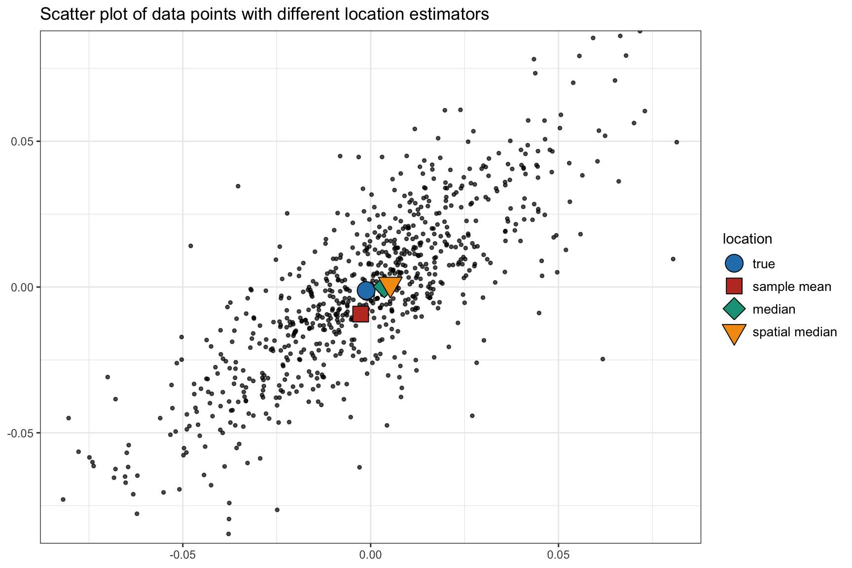
Figure 3.3: Illustration of different location estimators.
Figure 3.4 shows the estimation error of different location estimators as a function of the number of observations \(T\) for synthetic Gaussian and heavy-tailed data (the mean vector \(\bmu\) and covariance matrix \(\bSigma\) are taken as measured in typical stock market data). For Gaussian data, the sample mean is the best estimator (as further analyzed in Section 3.4), with the spatial median almost identical, and the elementwise median being the worst. For heavy-tailed data, the sample mean is as bad as the median and the spatial median remains the best. Overall, the spatial median seems to be the best option as it is robust to outliers and does not underperform under Gaussian data.
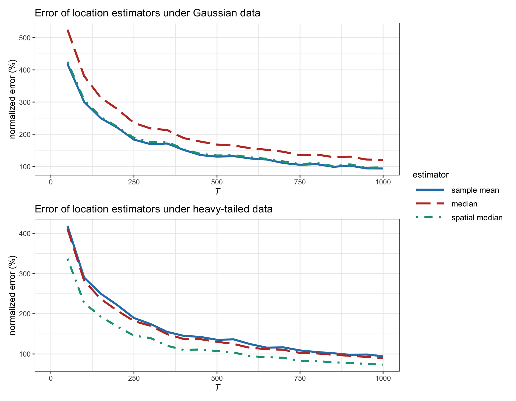
Figure 3.4: Estimation error of location estimators vs. number of observations (with \(N=100\)).
Figure 3.5 examines in more detail the effect of the heavy tails in the estimation error for synthetic data following a \(t\) distribution with degrees of freedom \(\nu\). Financial data typically corresponds to \(\nu\) on the order of somewhere between 4 and 5, which is significantly heavy-tailed, whereas a large value of \(\nu\) corresponds to a Gaussian distribution. We can observe that the error for the sample mean remains similar regardless of \(\nu\). Interestingly, the spatial median is similar to the sample mean for large \(\nu\) (Gaussian regime) whereas it becomes better for heavy tails. Again, this illustrates the robustness of the spatial median.
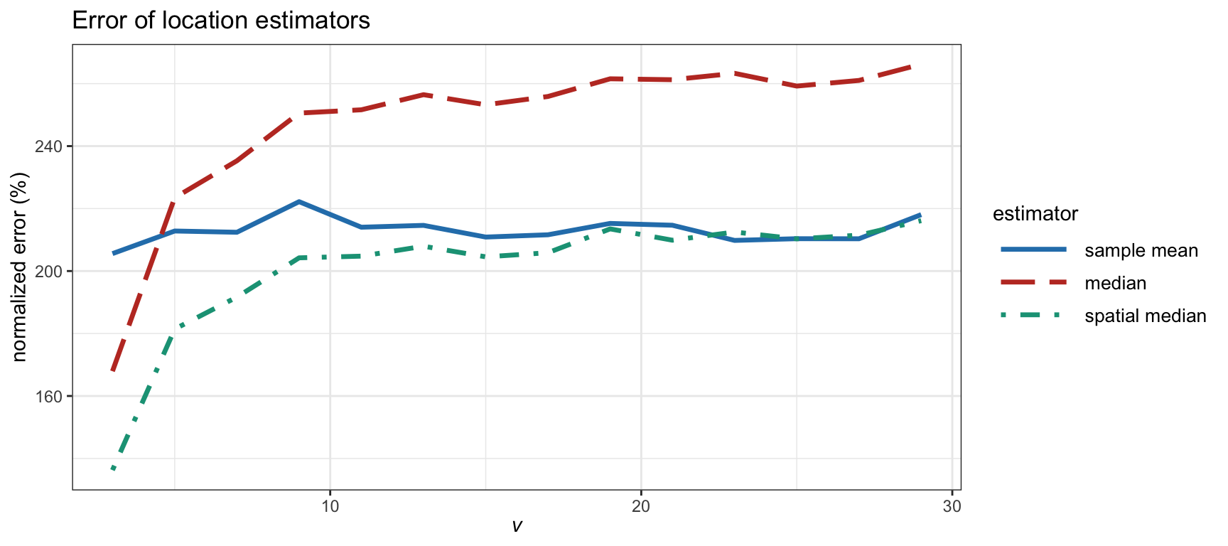
Figure 3.5: Estimation error of location estimators vs. degrees of freedom in a \(t\) distribution (with \(T=200\) and \(N=100\)).