2.5 Asset Structure
Apart from the structure along the temporal dimension, which can be used for modeling and forecasting, there is structure along the asset dimension (also referred to as cross-sectional structure). This means that rather than considering the assets one by one independently, they have to be jointly modeled.
This is particularly important when it comes to assessing the risk of a portfolio, since different stocks may have different correlations. For example, one may diversify an investment by allocating capital to several assets, but if they are strongly correlated it may not help in reducing the risk. Figure 2.25 illustrates the effect of asset correlation on the volatility of the equally weighted portfolio for the case of two assets with correlation \(\rho\) and each with variance 1. We can observe that for fully correlated assets, \(\rho=1\), the portfolio does not benefit from any diversity with respect to investing in a single asset and the variance remains at 1 (volatility of 1); for uncorrelated assets, \(\rho=0\), the portfolio gets a diversity benefit with the variance reduced to half (volatility of \(\sqrt{0.5}\)), and for negatively correlated assets, \(\rho < 0\), the diversity benefit increases further. In reality, assets tend to have a high correlation close to 1 and finding uncorrelated assets or classes of assets is the “holy grail.” The particular case of fully negatively correlated assets, \(\rho = -1\), can be achieved with a synthetic asset created for the sole purpose of hedging another one to control the risk exposure.
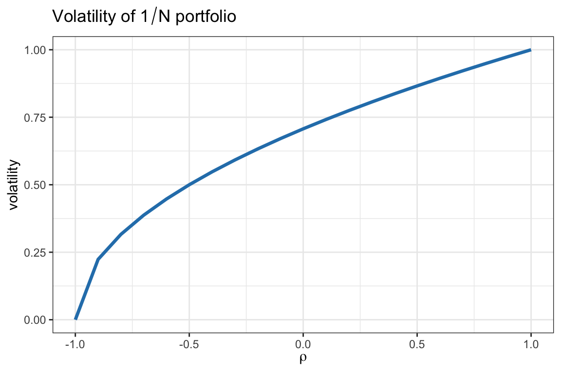
Figure 2.25: Effect of asset correlation on volatility for a two-asset portfolio.
Figure 2.26 shows heatmaps of the correlation matrix of some stocks from the S&P 500 (daily returns) and some cryptocurrencies (hourly returns). Compared to the diagonal elements (which are equal to 1), the off-diagonal components are much weaker (and no value lies in the negative range). In the case of cryptocurrencies, for example, there is a pair of names that are fully correlated: BTC and WBTC, which is expected since WBTC is by definition a wrapped BTC.
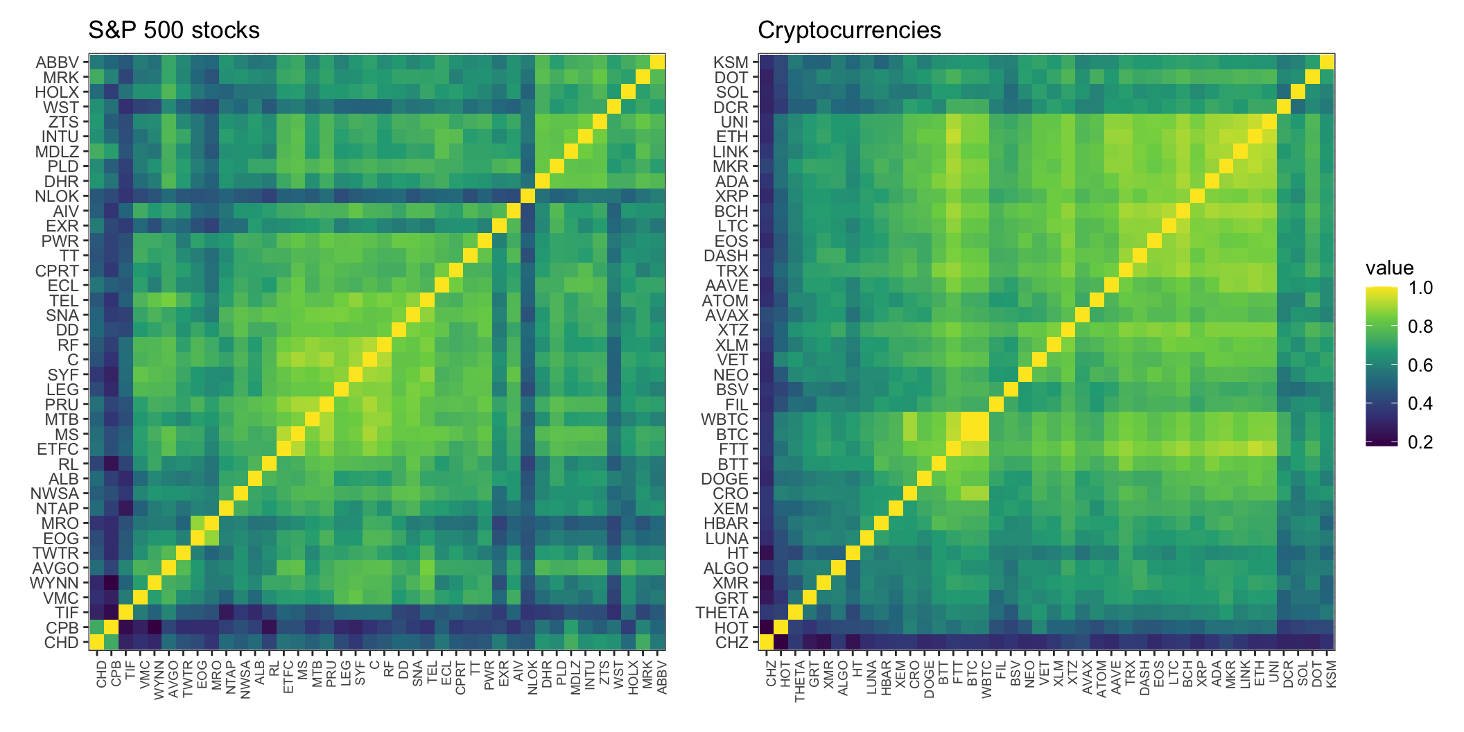
Figure 2.26: Correlation matrix of returns for stocks and cryptocurrencies.
We can confirm the previous observation that the cross-correlations are mostly nonnegative from the histograms depicted in Figure 2.27 for S&P 500 stocks (daily returns) and cryptocurrencies (hourly returns). In fact, this positive correlation among stocks and cryptocurrencies is not surprising since assets tend to move together with the market.
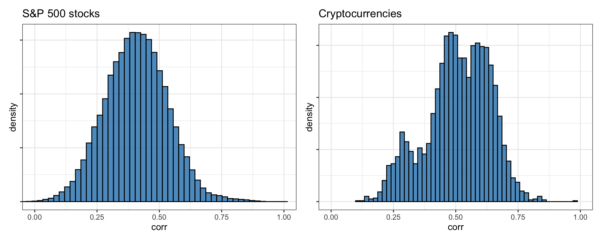
Figure 2.27: Histogram of correlations among returns of stocks and cryptocurrencies.
To explore the asset structure more deeply, it is worth inspecting how the eigenvalues of the correlation matrix tend to cluster into very few large ones and a big group of much smaller ones, the so-called factor model structure (Fama and French, 1992; Sharpe, 1964) (see Chapter 3 for details). Figure 2.28 depicts histograms of eigenvalues of the correlation matrix of daily returns for the S&P 500 stocks and hourly returns for the top 82 cryptocurrencies. In both cases, we can observe that a single eigenvalue is totally predominant (corresponding to the market index and constituting almost half of the total value of the eigenvalues), perhaps with one to four other nonnegligible eigenvalues, while the rest of them are orders of magnitude smaller (note that the horizontal axis follows a logarithmic scale).
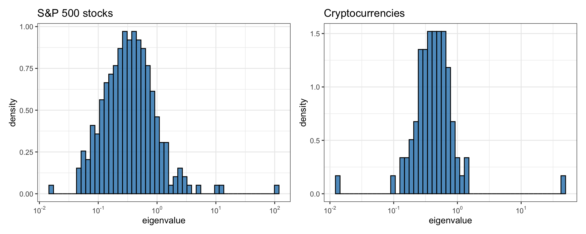
Figure 2.28: Histogram of correlation matrix eigenvalues of stocks and cryptocurrencies.