5.3 Learning Structured Graphs
The graph learning methods explored in Sections 5.2.2 and 5.2.3 can be successfully employed in different applications. Nevertheless, in some cases, some structural property of the unknown graph may be known and should be taken into account in the graph estimation process. Unfortunately, learning a graph with a specific structure is an NP-hard combinatorial problem for a general class of graphical models (Bogdanov et al., 2008) and, thus, designing a general algorithm is challenging.
Figure 5.7 illustrates different common types of graphs of interest, namely:
- multi-component or \(k\)-component graph: contains clusters, useful for classification;
- regular graph: where each node has the same number of neighbors (alternatively, the same degree), useful for balanced graphs;
- modular graph: satisfies some shortest path distance properties among triplets of nodes, useful for social network analysis;
- bipartite graph: containing two types of nodes with inter-connections and without intra-connections;
- grid graph: the nodes are distributed following a rectangular grid or two-dimensional lattice; and
- tree graph: undirected graph in which any two vertices are connected by exactly one path, resulting in a structure resembling a tree where connections branch out from nodes at each level.
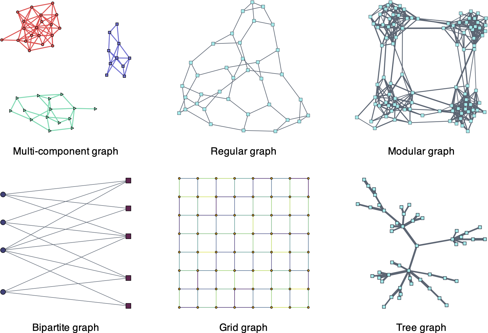
Figure 5.7: Types of structured graphs.
Some of the structural constraints are not difficult to control. For example, a grid graph simply means that each node can only be connected with a given neighborhood, that is, the adjacency and Laplacian matrices have many elements fixed to zero a priori. Another example is that of regular graphs where the degrees of the nodes, row sums of \(\bm{W}\), are fixed. If, instead, the number of neighbors is to be controlled, then the cardinality of the rows of \(\bm{W}\) has to be constrained, which is a nonconvex constraint.
However, other graph structural constraints are more complicated to control and can be characterized by spectral properties (i.e., properties on the eigenvalues) of the Laplacian and adjacency matrices (Chung, 1997). Such spectral properties can be enforced in the graph learning formulations (Kumar et al., 2019, 2020; Nie et al., 2016) as discussed next.
5.3.1 \(k\)-Component Graphs
A \(k\)-component graph (i.e., a graph with \(k\) clusters or components) is characterized by its Laplacian matrix being low rank with \(k\) zero eigenvalues (Chung, 1997).
More explicitly, consider the eigenvalue decomposition of the Laplacian matrix, \[\bm{L}=\bm{U}\textm{Diag}(\lambda_{1},\lambda_{2},\dots,\lambda_{p})\bm{U}^\T,\] where \(\bm{U}\) contains eigenvectors columnwise and \(\lambda_{1}\le\lambda_{2}\le\dots\le\lambda_{p}\) are the eigenvalues in increasing order. Then, a \(k\)-component graph has the \(k\) smallest eigenvalues equal to zero: \[ \lambda_{1} = \dots = \lambda_{k} = 0. \] The opposite direction is also true: if the Laplacian matrix has \(k\) zero eigenvalues, then it is a \(k\)-component graph. Figure 5.8 illustrates this spectral property of \(k\)-component graphs.
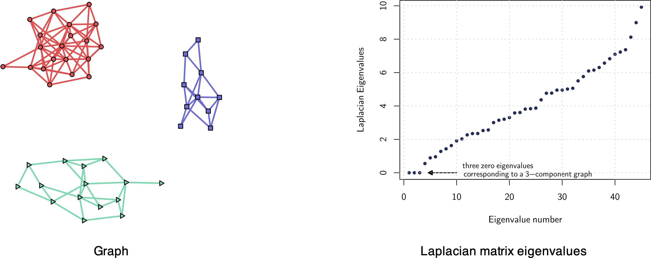
Figure 5.8: Example of a three-component graph (three clusters) with corresponding Laplacian matrix eigenvalues (three zero eigenvalues).
The low-rank property of the Laplacian matrix, \(\textm{rank}(\bm{L}) = p - k\), is a nonconvex and difficult constraint to handle in an optimization problem. In practice, it can be better handled by enforcing the sum of the \(k\) smallest eigenvalues to be zero, \(\sum_{i=1}^k \lambda_i(\bm{L}) = 0\), via Ky Fan’s theorem (Fan, 1949): \[ \sum_{i=1}^k \lambda_i(\bm{L}) = \underset{\bm{F}\in\R^{p\times k}:\bm{F}^\T\bm{F}=\bm{I}}{\textm{min}} \; \textm{Tr}(\bm{F}^\T\bm{L}\bm{F}), \] where the matrix \(\bm{F}\) becomes a new variable to be optimized.
For convenience, the low-rank constraint can be relaxed and moved to the objective function as a regularization term. For instance, denoting a general objective function by \(f(\bm{L})\), a regularized formulation could be \[ \begin{array}{ll} \underset{\bm{L},\bm{F}}{\textm{minimize}} & f(\bm{L}) + \gamma \textm{Tr}(\bm{F}^\T\bm{L}\bm{F})\\ \textm{subject to} & \textm{any constraint on } \bm{L},\\ & \bm{F}^\T\bm{F}=\bm{I}, \end{array} \] where now the optimization variables are \(\bm{L}\) and \(\bm{F}\), making the problem nonconvex due to the term \(\bm{F}^\T\bm{L}\bm{F}.\) To solve this problem we can conveniently use an alternate minimization between \(\bm{L}\) and \(\bm{F}\) (see Section B.6 in Appendix B for details). The optimization of \(\bm{L}\) with a fixed \(\bm{F}\) is basically the same problem without the low-rank structure, whereas the optimization of \(\bm{F}\) with a fixed \(\bm{L}\) is a trivial problem with a solution given by the eigenvectors corresponding to the \(k\) smallest eigenvalues of \(\bm{L}\).
Some illustrative and specific examples of low-rank graph estimation problems include:
- Low-rank graph approximation: Suppose we are given a graph in the form of a Laplacian matrix \(\bm{L}_0\); we can formulate the low-rank approximation problem as \[\begin{equation} \begin{array}{ll} \underset{\bm{L}\succeq\bm{0}, \bm{F}}{\textm{minimize}} & \|\bm{L} - \bm{L}_0\|_\textm{F}^2 + \gamma \textm{Tr}\left(\bm{F}^\T\bm{L}\bm{F}\right)\\ \textm{subject to} & \bm{L}\bm{1}=\bm{0}, \quad L_{ij} = L_{ji} \le 0, \quad \forall i\neq j,\\ & \textm{diag}(\bm{L})=\bm{1},\\ & \bm{F}^\T\bm{F}=\bm{I}. \end{array} \tag{5.8} \end{equation}\]
- Low-rank graphs from sparse GMRFs: Consider the formulation in (5.7) to learn a sparse Laplacian matrix under a GMRF framework. We can easily reformulate it to include a low-rank regularization term as \[\begin{equation} \begin{array}{ll} \underset{\bm{L}\succeq\bm{0}, \bm{F}}{\textm{maximize}} & \textm{log gdet}(\bm{L}) - \textm{Tr}(\bm{L}\bm{S}) - \rho\|\bm{L}\|_{0,\textm{off}} - \gamma \textm{Tr}\left(\bm{F}^\T\bm{L}\bm{F}\right)\\ \textm{subject to} & \bm{L}\bm{1}=\bm{0}, \quad L_{ij} = L_{ji} \le 0, \quad \forall i\neq j,\\ & \textm{diag}(\bm{L})=\bm{1},\\ & \bm{F}^\T\bm{F}=\bm{I}. \end{array} \tag{5.9} \end{equation}\] An alternative formulation based on \(\|\bm{L} - \bm{U}\bm{\Lambda}\bm{U}^\T\|_\textm{F}^2\) as the regularization term can also be considered (Kumar et al., 2019, 2020).24
Enforcing a low-rank Laplacian matrix will generate a \(k\)-component graph, but it may have isolated nodes. To avoid such trivial graph solutions one can control the degrees of the nodes with the constraint \(\textm{diag}(\bm{L})=\bm{1}\) (Cardoso and Palomar, 2020).
5.3.2 Bipartite Graphs
A bipartite graph is characterized by its adjacency matrix having symmetric eigenvalues around zero (Chung, 1997).
More explicitly, consider the eigenvalue decomposition of the adjacency matrix, \[\bm{W}=\bm{V}\textm{Diag}(\psi_1,\psi_2,\dots,\psi_p)\bm{V}^\T,\] where \(\bm{V}\) contains the eigenvectors columnwise and \(\psi_1\le\psi_2\le\dots\le\psi_p\) are the eigenvalues in increasing order. Then, a bipartite graph has symmetric eigenvalues around zero: \[\psi_i = -\psi_{p-i},\quad\forall i.\]
The opposite direction is also true: if the adjacency matrix has symmetric eigenvalues, then the graph is bipartite. Figure 5.9 illustrates this spectral property of bipartite graphs.
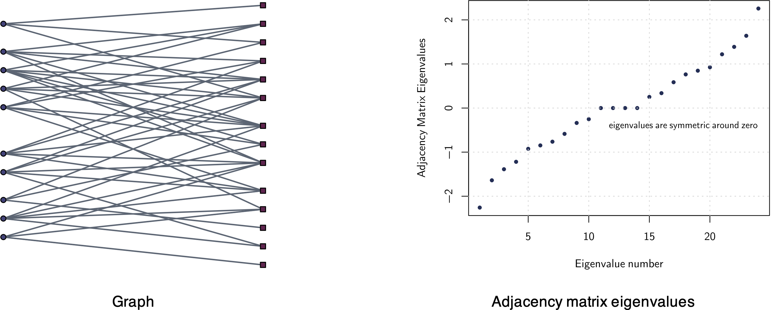
Figure 5.9: Example of a bipartite graph with corresponding adjacency matrix eigenvalues.
Enforcing symmetric eigenvalues in the adjacency matrix \(\bm{W}\) is a nonconvex and difficult constraint to handle in an optimization problem (Kumar et al., 2019, 2020). An alternative and more convenient characterization of a bipartite graph is via its Laplacian matrix, which has the following structure:25 \[\begin{equation} \bm{L} = \begin{bmatrix} \textm{Diag}(\bm{B}\bm{1}) & -\bm{B}\\ -\bm{B}^\T & \textm{Diag}(\bm{B}^\T\bm{1}) \end{bmatrix}, \tag{5.10} \end{equation}\] where \(\bm{B} \in \R_+^{r\times q}\) contains the edge weights between the two types of nodes (with \(r\) and \(q\) denoting the number of nodes in each group). Note that, any Laplacian \(\bm{L}\) constructed as in (5.10) already satisfies \(\bm{L}\bm{1}=\bm{0}, L_{ij} = L_{ji} \le 0, \forall i\neq j.\)
Some illustrative and specific examples of low-rank graph estimation problems are:
- Bipartite graph approximation: Suppose we are given a graph in the form of a Laplacian matrix \(\bm{L}_0\); we can find the closest bipartite graph approximation using (5.10) as \[ \begin{array}{ll} \underset{\bm{L},\bm{B}}{\textm{minimize}} & \|\bm{L} - \bm{L}_0\|_\textm{F}^2\\ \textm{subject to} & \bm{L} = \begin{bmatrix} \textm{Diag}(\bm{B}\bm{1}) & -\bm{B}\\ -\bm{B}^\T & \textm{Diag}(\bm{B}^\T\bm{1}) \end{bmatrix},\\ & \bm{B} \geq \bm{0}, \quad \bm{B}\bm{1}=\bm{1}. \end{array} \]
- Bipartite graphs from sparse GMRFs: Consider now the sparse GMRF formulation in (5.7), but enforcing the bipartite structure with (5.10) as follows (Cardoso et al., 2022a): \[\begin{equation} \begin{array}{ll} \underset{\bm{L}\succeq\bm{0}, \bm{B}}{\textm{maximize}} & \textm{log gdet}(\bm{L}) - \textm{Tr}(\bm{L}\bm{S}) - \rho\|\bm{L}\|_{0,\textm{off}}\\ \textm{subject to} & \bm{L} = \begin{bmatrix} \textm{Diag}(\bm{B}\bm{1}) & -\bm{B}\\ -\bm{B}^\T & \textm{Diag}(\bm{B}^\T\bm{1}) \end{bmatrix},\\ & \bm{B} \geq \bm{0}, \quad \bm{B}\bm{1}=\bm{1}. \end{array} \tag{5.11} \end{equation}\]
5.3.3 Numerical Experiments
For the empirical analysis, we again use three years’ worth of stock price data (2016–2019) from the following three sectors of the S&P 500 index: Industrials, Consumer Staples, and Energy.
Stocks are classified and grouped together into sectors and industries. This organization is convenient for investors in order to easily diversify their investment across different sectors (which presumably are less correlated than stocks within each sector). However, there are different criteria to classify stocks into sectors and industries, producing different classifications; for example:
- production-oriented approach: by the products they produce or use as inputs in the manufacturing process;
- market-oriented approach: by the markets they serve.
Table 5.1 lists some of the major sector classification systems in the financial industry:
GICS (Global Industry Classification Standard): A system developed by Morgan Stanley Capital International (MSCI) and Standard & Poor’s (S&P) in 1999 to classify companies and stocks into industry groups, sectors, and sub-industries based on their primary business activities.
ICB (Industry Classification Benchmark): A classification system developed by Dow Jones and FTSE Group that categorizes companies and securities into industries, supersectors, sectors, and subsectors based on their primary business activities. It is used by investors, analysts, and researchers for consistent sector analysis and performance comparison.
TRBC (Thomson Reuters Business Classification): A proprietary classification system developed by Thomson Reuters to categorize companies and securities into economic sectors, business sectors, and industries based on their primary business activities. It is used for research, analysis, and investment purposes.
In principle, each system is different and groups stocks in a different manner, although there is some degree of similarity.
| Level/System | GICS | ICB | TRBC |
|---|---|---|---|
| First | 11 sectors | 10 industries | 10 economic sectors |
| Second | 24 industry groups | 19 supersectors | 28 business sectors |
| Third | 68 industries | 41 sectors | 56 industry groups |
| Fourth | 157 sub-industries | 114 subsectors | 136 industries |
Given that there are multiple stock classifications into sectors and industries, it is not clear which one is more relevant in terms of portfolio investment. In a more data-oriented world, one can ignore such human-made classification systems and instead learn the graph of stocks from data and, perhaps, even enforce a \(k\)-component graph to obtain a clustered graph automatically.
Two-Stage vs. Joint Design of \(k\)-Component Graphs
Suppose we want to learn a \(k\)-component graph; as described in Section 5.3.1, one can employ two approaches:
Two-stage approach: First learn a connected graph using any formulation, such as the GMRF design in (5.6) or (5.7). Then perform a low-rank approximation to that graph as in (5.8).
Joint approach: Enforce the low-rank property in the GMRF formulation as in (5.9), which clearly must be better than the two-stage approach.
Figure 5.10 shows the effect of employing a joint design vs. the two-stage design using the GMRF formulation ((5.7) for the two-stage case and (5.9) for the joint case). The difference is too obvious to require any comment on the fact that a joint approach is significantly superior. Note, however, that care has to be taken with controlling the degrees when enforcing a low-rank graph, as discussed next.
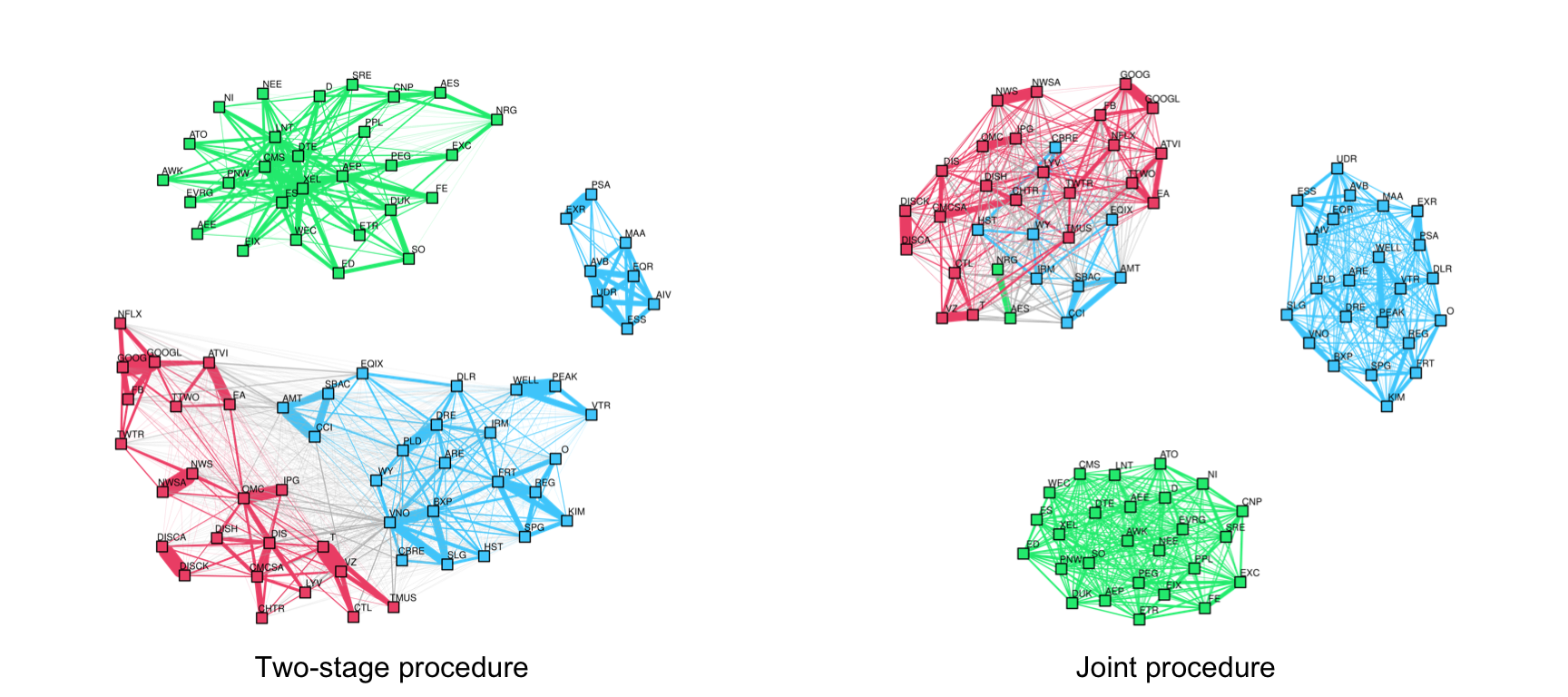
Figure 5.10: Effect of joint design vs. two-stage design on multi-component financial graphs.
Isolated Nodes in Low-Rank Designs for \(k\)-Component Graphs
Isolated nodes is an artifact that may happen when imposing a low-rank structure in the Laplacian matrix to obtain a graph with clusters. Basically, if one enforces a low-rank structure to learn a \(k\)-component graph but the graph deviates from a \(k\)-component graph, the solution to this formulation may trivially leave some nodes without any connection to other nodes (i.e., isolated nodes) to artificially increase the number of clusters.
The solution to avoid isolated nodes is quite simple. As discussed in Section 5.3.1, control the degrees of the nodes so that they are nonzero; even better if they are balanced.
Figure 5.11 clearly shows the effect of isolated nodes for the low-rank GMRF design in (5.9) and with the additional degree control. The difference is staggering: always control the degrees.
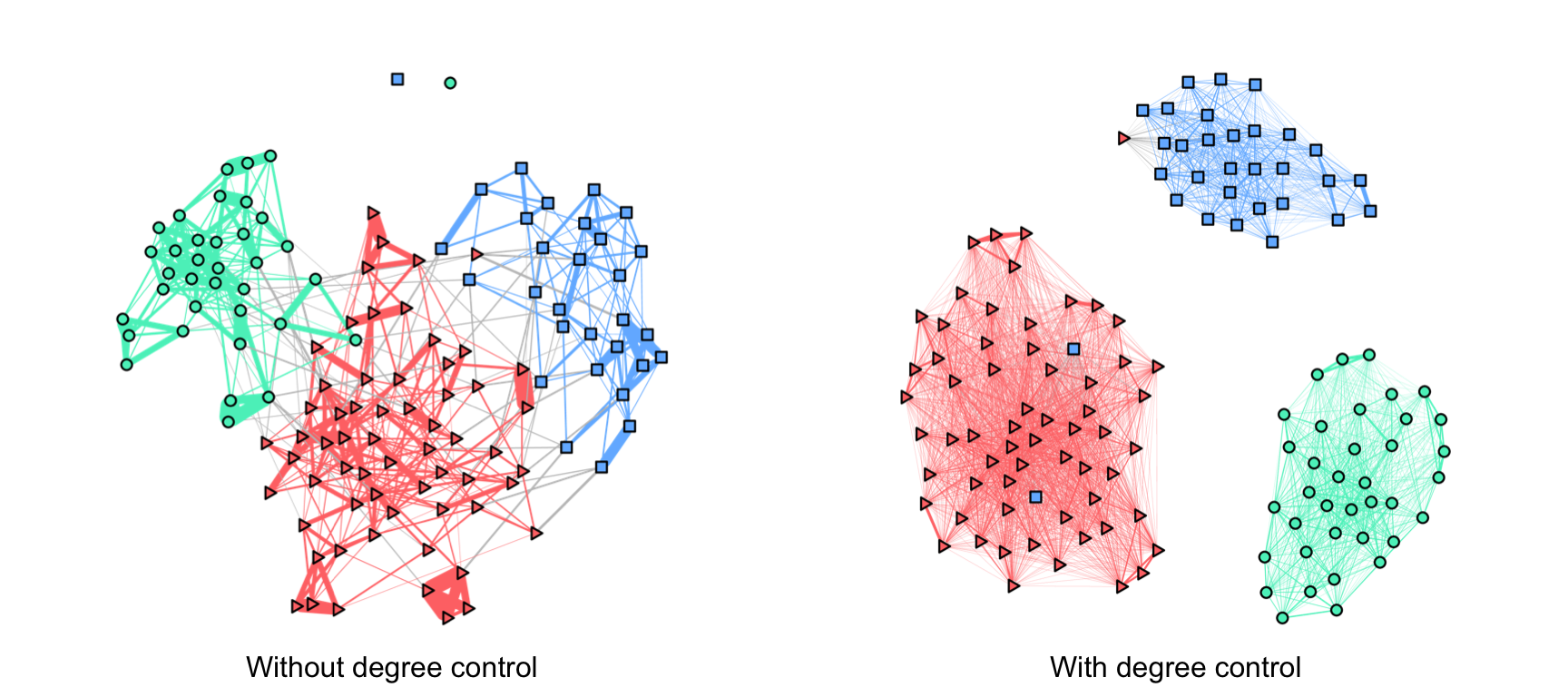
Figure 5.11: Effect of isolated nodes on low-rank (clustered) financial graphs.
References
The R package
spectralGraphTopologycontains several functions to solve graph formulations with spectral constraints (Cardoso and Palomar, 2022). ↩︎The R package
finbipartitecontains methods to solve problem (5.10) (Cardoso and Palomar, 2023a). ↩︎