5.4 Learning Heavy-Tailed Graphs
5.4.1 From Gaussian to Heavy-Tailed Graphs
The basic GMRF formulations in (5.6) or (5.7) are based on the assumption that data follow a Gaussian distribution, \[ f(\bm{x}) = \frac{1}{\sqrt{(2\pi)^N|\bSigma|}} \textm{exp}\left(-\frac{1}{2}(\bm{x} - \bmu)^\T\bSigma^{-1}(\bm{x} - \bmu)\right), \] leading to the maximum likelihood estimation of the Laplacian matrix \(\bm{L}\) (which plays the role of the inverse covariance matrix \(\bSigma^{-1}\)) formulated as \[\begin{equation} \begin{array}{ll} \underset{\bm{L}\succeq\bm{0}}{\textm{maximize}} & \textm{log gdet}(\bm{L}) - \textm{Tr}(\bm{L}\bm{S})\\ \textm{subject to} & \bm{L}\bm{1}=\bm{0}, \quad L_{ij} = L_{ji} \le 0, \quad \forall i\neq j. \end{array} \tag{5.12} \end{equation}\]
However, in many applications, data do not follow a Gaussian distribution. Instead, a better model for data may be a heavy-tailed distribution such as the Student \(t\) distribution characterized by \[ f(\bm{x}) \propto \frac{1}{\sqrt{|\bSigma|}} \left(1 + \frac{1}{\nu}(\bm{x} - \bmu)^\T\bSigma^{-1}(\bm{x} - \bmu)\right)^{-(p + \nu)/2}, \] where the parameter \(\nu>2\) determines how heavy the tails are (for \(\nu \rightarrow \infty\) it becomes the Gaussian distribution). This leads to \[\begin{equation} \begin{array}{ll} \underset{\bm{L}\succeq\bm{0}}{\textm{maximize}} & \begin{aligned}[t] \textm{log gdet}(\bm{L}) - \frac{p+\nu}{T}\displaystyle\sum_{t=1}^T \textm{log}\left(1 + \frac{1}{\nu}(\bm{x}^{(t)})^\T\bm{L}\bm{x}^{(t)}\right) \end{aligned} \\ \textm{subject to} & \bm{L}\bm{1}=\bm{0}, \quad L_{ij} = L_{ji} \le 0, \quad \forall i\neq j, \end{array} \tag{5.13} \end{equation}\] where the mean is assumed to be zero for simplicity.
This heavy-tailed formulation is nonconvex and difficult to solve directly. Instead, we can employ the majorization–minimization (MM) framework (Y. Sun et al., 2017) to iteratively solve the problem (see Section B.7 in Appendix B for details on MM). In particular, the logarithm upper bound \(\textm{log}(t) \leq \textm{log}(t_0) + \dfrac{t}{t_0} - 1\) leads to \[ \textm{log}\left(1 + \frac{1}{\nu}(\bm{x}^{(t)})^\T\bm{L}\bm{x}^{(t)}\right) \leq \textm{log}\left(1 + \frac{1}{\nu}(\bm{x}^{(t)})^\T\bm{L}_0\bm{x}^{(t)}\right) + \dfrac{\nu + (\bm{x}^{(t)})^\T\bm{L}\bm{x}^{(t)}}{\nu + (\bm{x}^{(t)})^\T\bm{L}_0\bm{x}^{(t)}} - 1. \]
Thus, the surrogate problem of (5.13) can be written similarly to the Gaussian case (Cardoso et al., 2021) as \[ \begin{array}{ll} \underset{\bm{L}\succeq\bm{0}}{\textm{maximize}} & \begin{aligned}[t] \textm{log gdet}(\bm{L}) - \frac{p + \nu}{T}\displaystyle\sum_{t=1}^T \dfrac{(\bm{x}^{(t)})^\T\bm{L}\bm{x}^{(t)}}{\nu + (\bm{x}^{(t)})^\T\bm{L}_0\bm{x}^{(t)}} \end{aligned}\\ \textm{subject to} & \bm{L}\bm{1}=\bm{0}, \quad L_{ij} = L_{ji} \le 0, \quad \forall i\neq j. \end{array} \]
Summarizing, the MM algorithm iteratively solves the following sequence of Gaussianized problems26 for \(k=1,2,\dots\): \[\begin{equation} \begin{array}{ll} \underset{\bm{L}\succeq\bm{0}}{\textm{maximize}} & \textm{log gdet}(\bm{L}) - \textm{Tr}(\bm{L}\bm{S}^k)\\ \textm{subject to} & \bm{L}\bm{1}=\bm{0}, \quad L_{ij} = L_{ji} \le 0, \quad \forall i\neq j, \end{array} \tag{5.14} \end{equation}\] where \(\bm{S}^k\) is conveniently defined as a weighted sample covariance matrix \[ \bm{S}^k = \frac{1}{T}\sum_{t=1}^T w_t^k \times \bm{x}^{(t)}(\bm{x}^{(t)})^\T, \] with weights \(w_t^k = \dfrac{p + \nu}{\nu + (\bm{x}^{(t)})^\T\bm{L}^k\bm{x}^{(t)}}\).
In words, to solve a heavy-tailed graph learning problem, instead of solving the Gaussian formulation in (5.12), one simply needs to solve a sequence of Gaussianized formulations as in (5.14).
5.4.2 Numerical Experiments
From Gaussian to Heavy-Tailed Graphs
We use again three years worth of stock price data (2016-2019) from the following three sectors of the S&P 500 index: Industrials, Consumer Staples, and Energy.
Figure 5.12 shows the results for the MRF formulations under the Gaussian assumption and under a heavy-tailed model. For the Gaussian case, the GMRF with a concave sparsity regularizer in (5.7) is used. For the non-Gaussian case, the heavy-tailed MRF formulation in (5.13) is employed. The conclusion is clear: heavy-tailed graphs are more convenient for financial data.
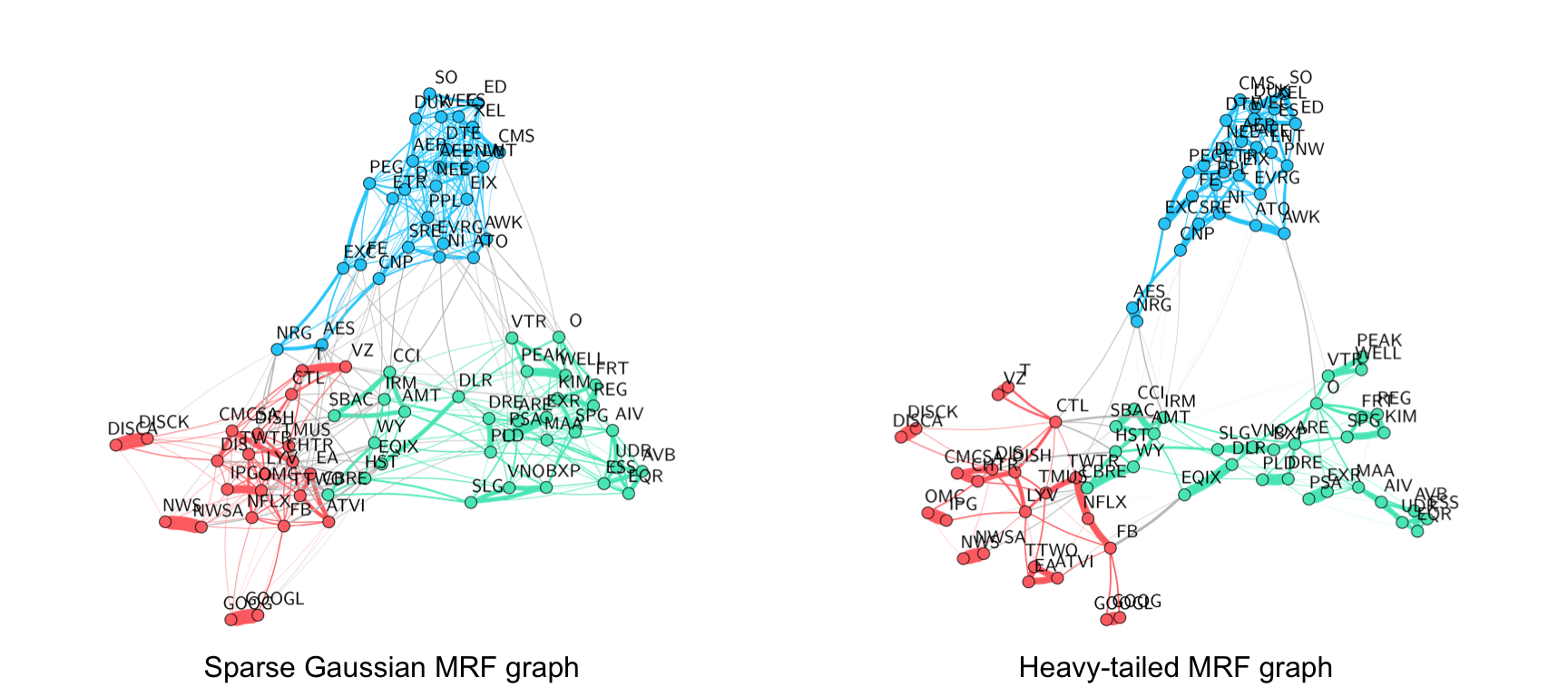
Figure 5.12: Gaussian vs. heavy-tailed graph learning with stocks.
\(k\)-Component Graphs
The effect of learning a \(k\)-component graph is that the graph will automatically be clustered. The following numerical example illustrates this point with foreign exchange (FX) market data (FX or forex is the trading of one currency for another). In particular, we use the 34 most traded currencies in the period from January 2, 2019 to December 31, 2020 (a total of \(n = 522\) observations). The data matrix is composed by the log-returns of the currency prices with respect to the United States dollar (USD). Unlike for S&P 500 stocks, there is no classification standard for currencies.
To start with, Figure 5.13 shows the graphs learned with the GMRF formulations (with the \(\ell_1\)-norm in (5.6) and concave sparsity regularizer in (5.7)) and with the heavy-tailed MRF formulation in (5.13). As expected, the GMRF graph with \(\ell_1\)-norm regularizer does not give a sparse graph like the one with a concave sparsity regularizer. Also, the heavy-tailed MRF formulation produces a much cleaner and more interpretable graph; for instance, the expected correlation between currencies of locations geographically close to each other is more evident, for example, {Hong Kong SAR, China}, {Taiwan, South Korea}, and {Poland, Czech Republic}.
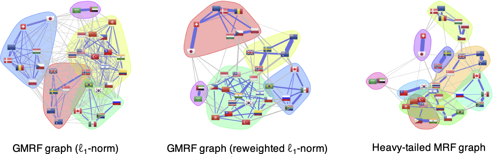
Figure 5.13: Gaussian vs. heavy-tailed graph learning with FX.
Turning now to \(k\)-component graphs, Figure 5.14 shows the equivalent graphs learned enforcing the low-rank structure to obtain clustered graphs (in particular, nine-component graphs). In this case, all the graphs are clearly clustered as expected. The heavy-tailed MRF graph provides a clearer interpretation with more reasonable clusters, such as {New Zealand, Australia} and {Poland, Czech Republic, Hungary}, which are not separated in the Gaussian-based graphs. Observe that the heavy-tailed MRF graph in (5.13) with low-rank structure controls the degrees of the nodes and isolated nodes are avoided (the GMRF formulations used do not control the degrees and the graphs present isolated nodes).
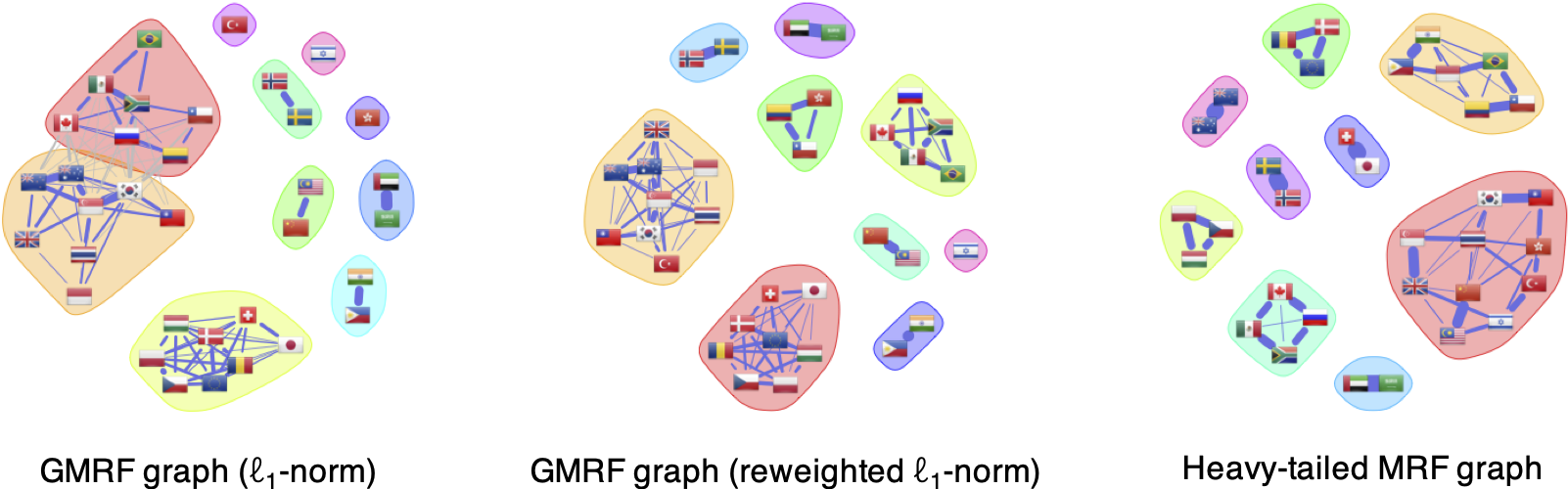
Figure 5.14: Gaussian vs. heavy-tailed multi-component graph learning with FX.
References
The R package
fingraph, based on Cardoso et al. (2021), contains efficient algorithms to learn graphs from heavy-tailed formulations (Cardoso and Palomar, 2023b). In particular, the functionlearn_regular_heavytail_graph()solves problem (5.13) with an additional degree constraint; also, the functionlearn_kcomp_heavytail_graph()further allows the specification of a \(k\)-component constraint. ↩︎