16.3 DL for portfolio design
In the context of portfolio design, deep learning can be used in a variety of ways. Recall that the two main components in portfolio design are data modeling and portfolio optimization. This is depicted in Figure 1.3 (Chapter 1) and reproduced herein for convenience in Figure 16.11.

Figure 16.11: Block diagram of data modeling and portfolio optimization.
In light of the block diagram in Figure 16.11, one could envision the usage of DL in at least three ways:
- using DL only in the modeling or time series forecasting component, while keeping the traditional portfolio optimization part;
- using DL only in the portfolio component, while keeping the traditional data modeling part; and
- using DL for both components, what is called end-to-end modeling.
We will not consider further the option of using DL only for the optimization part, since that is a well understood component that does not seem to require DL (in fact, this book has explored a wide variety of different portfolio formulations with efficient algorithms). Thus, we will focus on employing DL either in the forecast component or in the end-to-end system.
Regarding the input data to the DL system, one can use raw time series data, such as price data (e.g., open, high, low, close) and volume, as well as other alternative sources of data derived from technical analysis, fundamental analysis, macroeconomic data, financial statements, news, social media feeds, and investor sentiment analysis. Also, depending on the time horizon, a wide range of options for the frequency of the data may be available, varying from high frequency data and intraday price movements to daily, weekly, or even monthly stock prices.
16.3.1 Challenges
Before we explore the possibilities of DL for portfolio design, it is important to highlight the main challenges faced in this particular area. As already explained, deep neural networks have demonstrated an outstanding performance in many domain-specific areas, such as image recognition, natural language processing, board games and video games, biomedical applications, self-driving cars, etc. The million-dollar question is whether this revolution will extend to financial systems.
Since the 2010s, the financial industry and academia have been exploring the potential of DL in various applications, such as financial time series forecasting, algorithmic trading, risk assessment, fraud detection, portfolio management, asset pricing, derivatives market, cryptocurrency and blockchain studies, financial sentiment analysis, behavioral finance, and financial text mining. The number of research works keeps on increasing every year with an accelerated fashion, as well as open-source software libraries. However, we are just in the initial years of this new era and it is too early to say whether the success of DL enjoyed in non-financial applications will actually extend to financial systems and, particularly, to portfolio design.
Apart from very specific financial applications that have already enjoyed some success, such as sentiment analysis of news, credit default detection, or satellite image analysis for stock level estimation or crop production, we now focus on the potential of deep neural networks specifically for financial time series modeling and portfolio design. Among the many possible challenges that set these problems apart from other successful applications, the following ones are definitely worth mentioning:
Lack of data: Compared to other areas, such as natural language processing (e.g., GPT-3 was trained on a massive dataset of over 570 GB of text data), financial time series are in general extremely scarce (except for high-frequency data). For example, two years of daily stock prices amount to just 504 observations.
Low signal-to-noise ratio: The signal in financial data is extremely weak and totally submerged in noise. For example, an exploratory data analysis on asset returns corrected for the volatility envelope reveals a time series with little temporal structure (see Figures 2.23-2.24 in Chapter 2). On the other hand, an image of a cat typically has a high signal and very small noise (this is not to say that recognizing a cat is easy, but at least the signal-to-noise ratio is large).
Nonstationarity of data: Financial time series are clearly nonstationary (see Chapter 2) with a distribution that changes over time (e.g., bull markets, bear markets, side markets). This is in sharp contract with most other applications where DL has succeeded, in which the distribution remains constant: a cat stays the same, be it yesterday, today, or tomorrow.
Feedback adaptiveness of data: Financial data is totally influenced by human and machine decisions based on previous data. As a consequence, there exists a very unique feedback loop mechanism that cannot be ignored. In particular, once a pattern is discovered and a trading strategy is designed, this pattern tends to disappear in future data. Again, this is extremely different from other applications; for example, a cat remains a cat regardless of whether one can detect it in an image.
Lack of prior human evidence: In all the areas where DL has been successful, there was an obvious prior evidence of human performance that showed that the problem was solvable. For example, humans can easily recognize a cat, translate a sentence from English to Spanish, or drive a car. However, in finance there is no human who can effectively forecast the future performance of companies or trade a portfolio. Simply recall (see Chapter 13) the illustrative and clarifying statement (Malkiel, 1973): “a blindfolded chimpanzee throwing darts at the stock listings can select a portfolio that performs as well as those managed by the experts.”
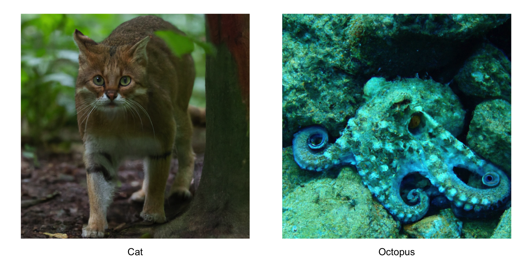
Figure 16.12: Can you spot the cat? And the octopus? Financial data is more like an octopus.
At the risk of oversimplifying, we could make a simple analogy of the problem of financial time series forecasting or portfolio design to that of identifying an octopus in an image, as opposed to the iconic example of identifying a cat in an image. This is exemplified in Figure 16.12. Indeed, this analogy seems to satisfy the previous list of challenges, namely:
- Lack of data: Arguably there are more images of cats than octopi in the human library of photos.
- Low signal-to-noise ratio: Think of a camouflaged octopus that looks exactly like the background (the octopus creates this noise to blend) as opposed to a domestic cat that stands out.
- Nonstationarity of data: Think again of an octopus that changes its camouflage over time (a cat’s appearance is the same today as it was yesterday).70
- Feedback adaptiveness of data: Think once more of an octopus that quickly adapts its camouflage as it is being chased by a predator (a cat is a cat).71
- Lack of prior human evidence: Humans are good at spotting domestic cats, but the same cannot be said about octopi.
We can finally summarize the previous analogy with the quote:72 “financial data ain’t cats, but octopi.”
16.3.2 Standard time series forecasting
By far the most common approach to employ DL in portfolio design is by using it in the time series modeling or forecasting component. This area has been intensively explored since 2015, as overviewed in (Sezer et al., 2020). LSTM, by its nature, utilizes the temporal characteristics of any time series signal due to its inherent memory. Thus, LSTM and its variations initially dominated the financial time series forecasting domain, e.g., (Fischer and Krauss, 2018). Nevertheless, more recently transformers have been shown to deal with long-term memory more efficiently.
The block diagram in Figure 16.13 illustrates the general process of time series forecasting. Following the machine learning paradigm in Figure 16.2, the input consists of a lookback of the past \(k\) time series values \(\left(\bm{x}_{t-k}, \dots,\bm{x}_{t-1}\right)\), the desired output or label is the next value of the time series \(\bm{x}_t\), and the produced output (i.e., the forecast) is denoted by \(\bmu_t\). With this, we can define some error measure between \(\bmu_t\) and \(\bm{x}_t\) to drive the learning process of the deep learning network. Note that the forecast horizon could be chosen further into the future instead of being just the next time index \(t\).

Figure 16.13: Block diagram of standard time series forecasting via DL.
The error measure that drives the learning process can be measured in a variety of ways. In a regression setting, the forecast value is a number or vector of values. We can then define the error vector \(\bm{e}_t = \bmu_t - \bm{x}_t\) and then compute quantities such as the mean square error (MSE), mean absolute error (MAE), median absolute deviation (MAD), mean absolute percentage error (MAPE), etc. In a classification setting, the forecast is the trend, e.g., up/down, and typical measures of error are the accuracy (i.e., correct prediction over total predictions), error rate (i.e., wrong predictions over total predictions), cross-entropy, etc. See (Goodfellow et al., 2016) for details.
Mathematically, the DL network implements the function \(\bm{f}_{\bm{\theta}}\left(\bm{x}_{t-k}, \dots,\bm{x}_{t-1}\right)\), with parameters \(\bm{\theta}\), to produce the estimate of \(\bm{x}_t\) as \(\bmu_t = \bm{f}_{\bm{\theta}}\left(\bm{x}_{t-k}, \dots,\bm{x}_{t-1}\right)\). The mathematical formulation of a standard time series forecasting can be written as the optimization problem \[ \begin{array}{ll} \underset{\bm{\theta}}{\textm{minimize}} & \E\left[\ell\left(\bm{f}_{\bm{\theta}}\left(\bm{x}_{t-k}, \dots,\bm{x}_{t-1}\right), \bm{x}_t\right)\right] \end{array} \] where \(\ell(\cdot, \cdot)\) denotes the prediction error function to be minimized (e.g., the MSE or cross-entropy).
It is important to point out that this architecture focuses on the time series modeling only, while totally ignoring the subsequent portfolio optimization component, which can also be taken into account as described next.
16.3.3 Portfolio-based time series forecasting
The previous standard time series modeling totally ignores the subsequent portfolio optimization component. As a consequence, the performance measure has to be defined in terms of an error that depends on the forecast \(\bmu_t\) and the label \(\bm{x}_t\). However, determining the most suitable error definition for the following portfolio optimization step is unclear and the choice is more heuristic.
Alternatively, a more holistic approach is to take into account the portfolio optimization component to measure the overall performance in a meaningful way, so that we do not need to reply on a rather arbitrary error definition.
The block diagram in Figure 16.14 illustrates this process of time series forecasting taking into account the subsequent portfolio optimization block in the training procedure (Bengio, 1997). Following the machine learning paradigm in Figure 16.3, instead of measuring an arbitrary error based on \(\bmu_t\) and \(\bm{x}_t\) to drive the learning process, the output \(\bmu_t\) is fed into the subsequent portfolio optimization block to produce the portfolio \(\bm{w}_t\), from which a meaningful measure of performance can be evaluated, such as the Sharpe ratio.

Figure 16.14: Block diagram of portfolio-based time series forecasting via DL.
Mathematically, the DL network implements the function \(\bm{f}_{\bm{\theta}}\left(\bm{x}_{t-k}, \dots,\bm{x}_{t-1}\right)\), with parameters \(\bm{\theta}\), to produce the estimate of \(\bm{x}_t\) as \(\bmu_t = \bm{f}_{\bm{\theta}}\left(\bm{x}_{t-k}, \dots,\bm{x}_{t-1}\right)\) (possibly also the corresponding covariance matrix \(\bSigma_t\)), from which the portfolio \(\bm{w}_t\) will be designed by minimizing some objective function \(f_0(\cdot)\) (following any of the portfolio formulations designs covered in this book). The mathematical formulation of a portfolio-based time series forecasting can be written as the optimization problem \[ \begin{array}{ll} \underset{\bm{\theta}}{\textm{minimize}} & \E\left[\xi\left(\bm{w}_t, \bm{x}_t\right)\right]\\ \textm{subject to} & \bm{w}_t = \underset{\bm{w}}{\textm{arg min}} \; f_0\left(\bm{w}; \bmu_t = \bm{f}_{\bm{\theta}}\left(\bm{x}_{t-k}, \dots,\bm{x}_{t-1}\right)\right), \end{array} \] where \(\xi(\cdot, \cdot)\) denotes the error function to be minimized that measures the overall system performance (e.g., the negative of the Sharpe ratio). Note that in this approach, the parameters of the DL network \(\bm{\theta}\) are optimized to minimize directly the overall system performance instead of a simple forecasting error, such as the MSE or the cross-entropy. In principle, one may use \(f_0 = \xi\), i.e., use the same criterion to design the portfolio as the one used to measure the overall performance; however, there may be reasons to actually use a different criterion.
The difficulty of this architecture is in the learning process. To be more specific, the backpropagation learning algorithm requires the computation of the partial derivatives of the output of each block with respect to its input (to be used in the chain rule for differentiation). If the portfolio optimization block has a closed-form expression, e.g., \(\bm{w}_t = \bSigma_t^{-1}\bmu_t\), then the partial derivatives are trivially computed. However, if this block is defined in terms of the solution to an optimization problem, then it becomes trickier since one has to be able to compute the partial derivatives of the solution via the KKT optimality conditions (see Section A.6.4 in Appendix A) of the optimization problem. Fortunately, recent developments have made this possible and available in open-source libraries (Amos and Kolter, 2017).
It is important to note that in this architecture, the time series forecast not only produces the forecast vector \(\bmu_t\) but also a measure of the uncertainty of the forecast in the form of the covariance matrix \(\bSigma_t\). This is necessary since the subsequent portfolio optimization component may need both \(\bmu_t\) and \(\bSigma_t\).
16.3.4 End-to-end portfolio design
The DL portfolio-based time series forecasting architecture in Figure 16.14 is an improvement over the standard time series forecasting architecture in Figure16.13, because it takes into account the subsequent portfolio optimization block and measures the overall performance using a meaningful performance measure.
However, since DL has proven to be such a powerful universal function approximator in many other areas, we can also consider a more bold architecture commonly termed end-to-end design, where the whole process is modeled by a single DL component as illustrated in Figure 16.15.

Figure 16.15: Block diagram of end-to-end portfolio design via DL.
Mathematically, the end-to-end DL network implements the function \(\bm{f}_{\bm{\theta}}\left(\bm{x}_{t-k}, \dots,\bm{x}_{t-1}\right)\), with parameters \(\bm{\theta}\), to produce directly the portfolio \(\bm{w}_t\) (without going through an intermediate forecasting block). The formulation of this end-to-end DL portfolio can be written as \[ \begin{array}{ll} \underset{\bm{\theta}}{\textm{minimize}} & \E\left[\xi\left(\bm{w}_t, \bm{x}_t\right)\right]\\ \textm{subject to} & \bm{w}_t = \bm{f}_{\bm{\theta}}\left(\bm{x}_{t-k}, \dots,\bm{x}_{t-1}\right), \end{array} \] where \(\xi(\cdot, \cdot)\) denotes the error function to be minimized that measures the overall system performance (e.g., the negative of the Sharpe ratio).
In principle, this end-to-end architecture is the most powerful one, because it can learn to optimize the overall performance measure of interest. However, this comes at the price of requiring huge amounts of data. The reason is that an end-to-end architecture needs to be deep enough to properly optimize the performance measure, which implies more weights to be learned and more data. In financial applications, we may not have this luxury of huge amounts of data. Thus, it is not clear yet whether an end-to-end design is feasible in practice.
16.3.5 Reinforcement learning end-to-end portfolio design
As previously discussed, in order to have a really powerful DL architecture, it has to be deep enough in terms of layers, which requires huge amounts of training data. This means that such data-hungry architectures may be more suitable for high-frequency data applications, such as high-frequency trading (HFT). But this potential scenario also comes at a price.
A critical aspect of HFT is that the portfolio designed and executed in the market may severely affect the state of the market due to the so-called market impact. The market impact depends on the liquidity of the assets, but in HFT liquidity is much smaller and the slippage becomes too important to be ignored.
This situation in which the actions of the agent affect the state of the system falls into another machine learning paradigm different from supervised learning called reinforcement learning (RL). In RL, algorithms engage with the environment, creating a feedback loop between the learning system and its experiences. The learning in such systems cannot be done before hand (as in supervised learning) and has to be implemented in an online fashion, i.e., as the orders are executed the system learns in real time. One can expect that the learning will be slower under this paradigm, so again it is not clear whether this could be useful in a portfolio strategy context. A comprehensive overview of research efforts on RL-based methods for quantitative trading is given in (S. Sun et al., 2023).
References
Cats, like all living creatures, do evolve, but they do so on an evolutionary time scale of, say, millions of years. So, for practical purposes we can assume them fixed.↩︎
Cats, like most animals, have evolved camouflage to avoid predators, but cannot adapt it to the changing environment in real time, unlike other species like octopus, squid, and chameleon.↩︎
The cat versus octopus comparison is just an analogy for illustration purposes. This is not to say that DL cannot literally be trained to spot an octopus.↩︎