10.4 Tail portfolios (CVaR and EVaR)
We will now focus of CVaR and EVaR portfolios (and the limiting case of the worst-case portfolio) since they can be conveniently formulated as convex problems.
10.4.1 Formulation for CVaR portfolios
The mean–CVaR formulation replaces the usual variance term \(\w^\T\bSigma\w\) by the CVaR in (10.4) as a measure of risk: \[\begin{equation} \begin{array}{ll} \underset{\w}{\textm{maximize}} & \w^\T\bmu - \lambda \, \textm{CVaR}_{\alpha}(\w)\\ \textm{subject to} & \w \in \mathcal{W}. \end{array} \tag{10.9} \end{equation}\] As usual, this problem can be similarly formulated by moving either the expected return or risk term to the constraints (see Chapter 7).
To write the problem in convex form, we will use the variational convex representation of the CVaR in (10.6): \[ \textm{CVaR}_{\alpha}(\w) = \underset{\tau}{\textm{inf}} \left\{\tau + \frac{1}{1-\alpha}\E\left[(-\w^\T\bm{r}-\tau)^+\right]\right\}. \] This leads to the convex mean–CVaR formulation: \[ \begin{array}{ll} \underset{\w, \tau}{\textm{maximize}} & \w^\T\bmu - \lambda \left(\tau + \frac{1}{1-\alpha}\E\left[(-\w^\T\bm{r}-\tau)^+\right]\right)\\ \textm{subject to} & \w \in \mathcal{W}, \end{array} \] where the auxiliary variable \(\tau\) has been conveniently moved from the inner minimization to the outer maximization (and we have tacitly assumed that the set \(\mathcal{W}\) is convex).
In practice, the expectation operator is approximated by the sample mean over \(T\) observations \(\bm{r}_1, \dots, \bm{r}_T\): \[ \E\left[(-\w^\T\bm{r}-\tau)^+\right] \approx \frac{1}{T}\sum_{t=1}^T (-\w^\T\bm{r}_t - \tau)^+. \]
Thus, the mean–CVaR formulation is finally given as \[ \begin{array}{ll} \underset{\w, \tau}{\textm{maximize}} & \w^\T\bmu - \lambda \left(\tau + \frac{1}{1-\alpha} \frac{1}{T}\sum_{t=1}^T (-\w^\T\bm{r}_t - \tau)^+ \right)\\ \textm{subject to} & \w \in \mathcal{W}. \end{array} \]
From an optimization perspective, it is convenient to rewrite the formulation without the nondifferentiable operator \((\cdot)^+\) by introducing the \(T\) auxiliary variables \(\bm{u}=(u_1,\dots,u_T)\) as \[\begin{equation} \begin{array}{ll} \underset{\w, \tau, \bm{u}}{\textm{maximize}} & \w^\T\bmu - \lambda \left(\tau + \frac{1}{1-\alpha} \frac{1}{T}\sum_{t=1}^T u_t \right)\\ \textm{subject to} & 0 \le u_t \ge -\w^\T\bm{r}_t - \tau, \qquad t=1,\dots,T\\ & \w \in \mathcal{W}. \end{array} \tag{10.10} \end{equation}\] This problem is a linear program (assuming that the set \(\mathcal{W}\) is described via linear constraints) and can be conveniently solved with an LP solver.
It is important to bear in mind that the tail events in the CVaR formulation (10.10) happen with low probability (by definition) and, therefore, very few samples (if any) will contribute to the characterization of the CVaR. For instance, if \(\alpha=0.99\) and we have \(T=200\) observations, then only 2 samples out of the 200 will characterize the tail, which are too few samples for a proper characterication of the shape of the tail. This effect is further exarcerbated as the dimension \(N\) becomes large. As a consequence, the CVaR portfolio may not be numerically stable and alternative methods have been proposed, such as based on some parametric distribution of the returns (Gaussian or elliptical distributions), alternative estimation methods for CVaR (Hong et al., 2014; Nadarajah et al., 2014), use of worst-case characterizations of CVaR (Zhu and Fukushima, 2009), and sophisticated tail characterizations based on extreme value theory (McNeil and Frey, 2000).
10.4.2 Formulation for EVaR portfolios
Similarly to (10.11), the mean–EVaR formulation replaces the usual variance term \(\w^\T\bSigma\w\) by the EVaR in (10.5) as a measure of risk: \[\begin{equation} \begin{array}{ll} \underset{\w}{\textm{maximize}} & \w^\T\bmu - \lambda \, \textm{EVaR}_{\alpha}(\w)\\ \textm{subject to} & \w \in \mathcal{W}. \end{array} \tag{10.11} \end{equation}\]
Using the change of variable \(t=z^{-1}\) in the EVaR (10.5), the problem can be written (Ahmadi-Javid and Fallah-Tafti, 2019) as \[ \begin{array}{ll} \underset{\w, t>0}{\textm{maximize}} & \w^\T\bmu - \lambda \left(t\;\textm{log}\left(\frac{1}{1-\alpha}\E\left[\textm{exp}(-t^{-1}\w^\T\bm{r})\right]\right)\right)\\ \textm{subject to} & \w \in \mathcal{W}, \end{array} \] which is a convex problem (assuming that the set \(\mathcal{W}\) is convex) because the log-sum-exp function is convex and the perspective \(tf(\bm{x}/t)\) of a function \(f(\bm{x})\) preserves convexity (see Appendix A for details on convexity).
In practice, the expectation operator is approximated by the sample mean over \(T\) observations \(\bm{r}_1, \dots, \bm{r}_T\) and the mean–EVaR formulation is finally written as \[\begin{equation} \begin{array}{ll} \underset{\w, t>0}{\textm{maximize}} & \w^\T\bmu - \lambda \left( t\;\textm{log}\left(\sum_{t'=1}^T\left[\textm{exp}(-t^{-1}\w^\T\bm{r}_{t'})\right]\right) - t\;\textm{log}\left((1-\alpha)T\right) \right)\\ \textm{subject to} & \w \in \mathcal{W}. \end{array} \tag{10.12} \end{equation}\]
This problem can be solved in practice in a variety of ways (see Appendix B for a discussion on algorithms, solvers and modeling frameworks), namely:
via a general-purpose solver (since the problem is convex, it will find an optimal solution);
via a tailored interior-point method for convex problems (Ahmadi-Javid and Fallah-Tafti, 2019);
via a convex modeling framework that can recognize the convexity of the log-sum-exp function and then performing bisection over \(t\);
via a convex modeling framework that can recognize both the convexity of the log-sum-exp function and the convexity-preserving property of the perspective operator;
via a convex reformulation in terms of the exponential cone \(\mathcal{K}_{\textm{exp}}\) (Chares, 2007),47 which some solvers and modeling frameworks can recognize (Dany Cajas, 2021a):48 \[ \begin{array}{ll} \underset{\w, t>0, s, \bm{u}}{\textm{maximize}} & \w^\T\bmu - \lambda \left(s - t\;\textm{log}\left((1-\alpha)T\right) \right)\\ \textm{subject to} & \w \in \mathcal{W}\\ & t \ge u_1 + \dots + u_T\\ & (-\w^\T\bm{r}_{t'} - s, t, u_{t'}) \in \mathcal{K}_{\textm{exp}}, \quad t'=1,\dots,T, \end{array} \] where \[ \mathcal{K}_{\textm{exp}} \triangleq \big\{(a,b,c) \mid c\geq b\,e^{a/b}, b>0\big\} \cup \big\{(a,b,c) \mid a\leq0, b=0, c\geq0\big\}. \]
10.4.3 Formulation for the worst-case portfolio
The VaR, CVaR, and EVaR all tend to the maximal value of the support of the pdf of the loss as \(\alpha \rightarrow 1\). In practice, this implies focusing the attention to the worst realization of the return or loss.
This worst-case risk leads to the following formulation (M. R. Young, 1998): \[ \begin{array}{ll} \underset{\w}{\textm{maximize}} & \w^\T\bmu - \lambda\; \textm{max}_{1\le t\le T}\{-\w^\T\bm{r}_t\}\\ \textm{subject to} & \w \in \mathcal{W} \end{array} \] or, without the nondifferentiable maximum operator, as \[\begin{equation} \begin{array}{ll} \underset{\w, \tau}{\textm{maximize}} & \w^\T\bmu - \lambda\; \tau\\ \textm{subject to} & \tau \ge -\w^\T\bm{r}_t, \qquad t=1,\dots,T\\ & \w \in \mathcal{W}. \end{array} \tag{10.13} \end{equation}\] This problem is again a linear program (assuming that the set \(\mathcal{W}\) is described via linear constraints) and can be conveniently solved with an LP solver.
10.4.4 Numerical experiments
We now compare CVaR, EVaR, and worst-case portfolios based on (10.10), (10.12), and (10.13), respectively. To focus on the effect of the risk measure, we ignore the expected return term in the optimization (effectively letting \(\lambda\rightarrow\infty\)) and also include the GMVP as a reference benchmark.
A word of caution is necessary. Since these portfolio formulations are based on a non-parametric computation of the risk (observed returns directly instead of some covariance matrix) and the tail events happen with low probability (by definition), we cannot expect a good characterization of the true tail. The most extreme case is the worst-case portfolio which is defined by a single data point. For the CVaR, very few observations (if any) may occur on the tail, and this can be exacerbated with larger values of \(\alpha\). The EVaR may be slightly better in this regard since it uses all the observations. For this reason, alternative more stable methods have been proposed, as previously mentioned, based on parametric models or sophisticated tail characterizations based on extreme value theory.
Figure 10.6 shows boxplots of the Sharpe ratio and maximum drawdown for 200 realizations of 50 randomly chosen stocks, from the S&P 500 during 2015-2020, reoptimizing the portfolios every month with a lookback of one year. It is difficult to draw conclusions from this numerical experiment, but the EVaR portfolios seem to produce better results than the CVaR ones as expected.
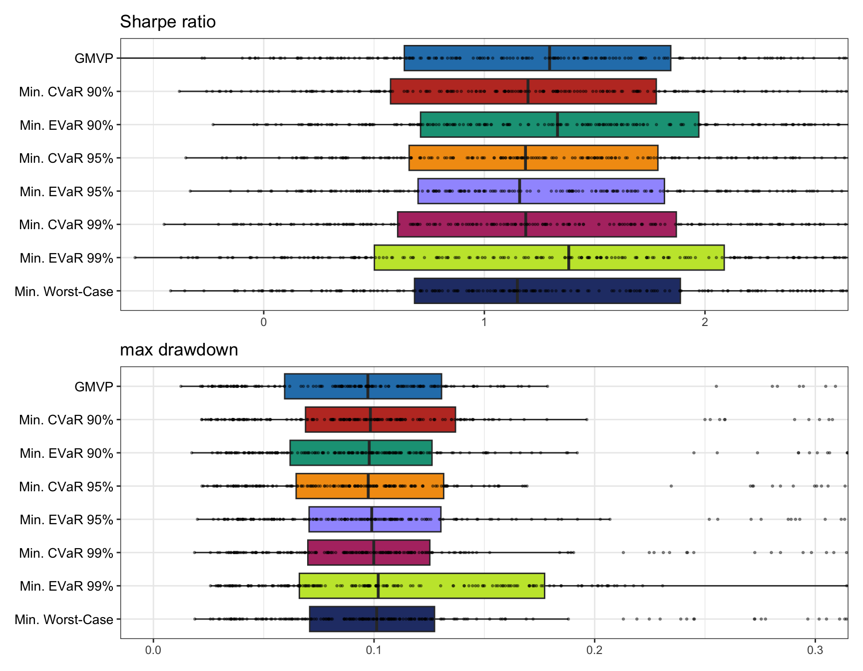
Figure 10.6: Backtest performance of CVaR and EVaR portfolios.
References
The following convex constraint involving the log-sum-exp function \[ s \ge t\; \textm{log}\left( e^{x_1/t} + e^{x_2/t} \right), \] for \(t>0\), can be rewritten in terms of the exponential cone \(\mathcal{K}_{\textm{exp}}\) as (Chares, 2007) \[ \begin{aligned} t & \ge u_1 + u_2\\ (x_i - s, t, u_i) & \in \mathcal{K}_{\textm{exp}}, \qquad i=1,2. \end{aligned} \]↩︎
Some solvers like the Embedded COnic Solver (ECOS) solver (https://github.com/embotech/ecos) or MOSEK (https://www.mosek.com) are able to handle problems with the exponential cone. Some modeling frameworks like CVXR (https://cvxr.rbind.io) can also accept the exponential cone.↩︎