3.1 IID model
Chapter 2 gives an exploratory view of financial data and the important stylized facts. This chapter explores a simple but useful and popular way to model financial data. Suppose we have \(N\) securities or tradable assets—possibly from distinct asset classes such as bonds, equities, commodities, mutual funds, currencies, and cryptos—and let \(\bm{x}_t\in\R^N\) (often denoted as \(\bm{r}_t\)) denote the random returns of the assets at time \(t\). Note that the time index \(t\) can denote any arbitrary period such as minutes, hours, days, weeks, months, quarters, years, etc.
Under the i.i.d. model, the returns are simply modeled as \[\begin{equation} \bm{x}_t = \bmu + \bm{\epsilon}_t, \tag{3.1} \end{equation}\] where \(\bmu\in\R^N\) denotes the expected return and \(\bm{\epsilon}_t\in\R^N\) is the residual component with zero mean and covariance matrix \(\bSigma\in\R^{N\times N}\). This model can be motivated by the efficient-market hypothesis (Fama, 1970).9 Figure 3.1 shows an example of a synthetic univariate Gaussian i.i.d. time series.
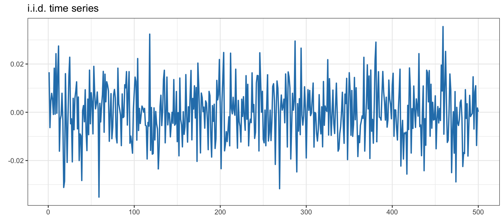
Figure 3.1: Example of a synthetic Gaussian i.i.d. time series.
To be more exact, the i.i.d. model in (3.1) corresponds to the random walk model (Campbell et al., 1997; Malkiel, 1973) on the log-prices \(\bm{y}_t \triangleq \textm{log}\; \bm{p}_{t}\) (also referred to as geometric random walk model on the prices): \[ \bm{y}_{t} = \bmu + \bm{y}_{t-1} + \bm{\epsilon}_t, \] which leads to (3.1) when \(\bm{x}_t\) denotes the log-returns: \(\bm{x}_t = \bm{y}_t - \bm{y}_{t-1}.\)
The i.i.d. model in (3.1) ignores any temporal structure or dependency in the data. Chapter 4 considers more sophisticated time series models that attempt to incorporate the time structure. Some accessible textbooks that cover financial data modeling are (Meucci, 2005; Ruppert and Matteson, 2015; Tsay, 2010), with more emphasis on the multivariate case in (Lütkepohl, 2007; Tsay, 2013).
References
Eugene F. Fama was awarded the 2013 Sveriges Riksbank Prize in Economic Sciences in Memory of Alfred Nobel for his work on the efficient-market hypothesis (EMH). Ironically, Robert J. Shiller was co-awarded the same prize precisely for his work on the inefficiency of markets. ↩︎