第 36 章 tidyverse中的若干技巧
聊聊tidyverse中常用的一些小技巧
“most of data science is counting, and sometimes dividing” — Hadley Wickham
36.1 count()
我之前多次用到count()函数,其功能就是统计某个变量中各组出现的次数
df <- tibble(
  name = c("Alice", "Alice", "Bob", "Bob", "Carol", "Carol"),
  type = c("english", "math", "english", "math", "english", "math"),
  score = c(60.2, 90.5, 92.2, 98.8, 82.5, 74.6)
)

df
## # A tibble: 6 × 3
## name type score
## <chr> <chr> <dbl>
## 1 Alice english 60.2
## 2 Alice math 90.5
## 3 Bob english 92.2
## 4 Bob math 98.8
## 5 Carol english 82.5
## 6 Carol math 74.6## # A tibble: 3 × 2
## name n
## <chr> <int>
## 1 Alice 2
## 2 Bob 2
## 3 Carol 2如果用之前讲的group_by() + summarise()来写,
## # A tibble: 3 × 2
##   name      n
##   <chr> <int>
## 1 Alice     2
## 2 Bob       2
## 3 Carol 2count() 还有更多强大的参数, 比如
## # A tibble: 3 × 2
##   name  total_score
##   <chr>       <dbl>
## 1 Bob          191
## 2 Carol        157.
## 3 Alice 151.如果不用count(),用group_by() + summarise()写,
df %>%
  group_by(name) %>%
  summarise(
    n = n(),
    total_score = sum(score, na.rm = TRUE)
  ) %>%
  arrange(desc(total_score))
## # A tibble: 3 × 3
## name n total_score
## <chr> <int> <dbl>
## 1 Bob 2 191
## 2 Carol 2 157.
## 3 Alice 2 151.当然,count()在特定场合下的简便写法,遇到复杂的分组统计,还是得用用group_by() + summarise()组合。
36.2 在 count() 中创建新变量
可以在count()里构建新变量,并利用这个新变量完成统计
## # A tibble: 4 × 2
##   range     n
##   <dbl> <int>
## 1    60     1
## 2    70     1
## 3    80     1
## 4    90     3
36.3 add_count()
想增加一列,代表每人参加的考试次数
## # A tibble: 6 × 4
##   name  type    score     n
##   <chr> <chr>   <dbl> <int>
## 1 Alice english  60.2     2
## 2 Alice math     90.5     2
## 3 Bob   english  92.2     2
## 4 Bob   math     98.8     2
## 5 Carol english  82.5     2
## 6 Carol math     74.6     2
可以有更简单的方法
## # A tibble: 6 × 4
##   name  type    score     n
##   <chr> <chr>   <dbl> <int>
## 1 Alice english  60.2     2
## 2 Alice math     90.5     2
## 3 Bob   english  92.2     2
## 4 Bob   math     98.8     2
## 5 Carol english  82.5     2
## 6 Carol math     74.6     2
36.4 nth(), first(), last()
v <- c("a", "c", "d", "k")
v[1]## [1] "a"
v[length(v)]## [1] "k"## [1] "d"## [1] "a"## [1] "k"用在数据框中,同样可以使用
## # A tibble: 1 × 3
##   name  type    score
##   <chr> <chr>   <dbl>
## 1 Alice english 60.2## # A tibble: 3 × 3
## # Groups: name [3]
## name type score
## <chr> <chr> <dbl>
## 1 Alice math 90.5
## 2 Bob math 98.8
## 3 Carol math 74.636.5 列变量重新排序
比如想把score放在第一列
df %>%
  select(score, everything())
## # A tibble: 6 × 3
## score name type
## <dbl> <chr> <chr>
## 1 60.2 Alice english
## 2 90.5 Alice math
## 3 92.2 Bob english
## 4 98.8 Bob math
## 5 82.5 Carol english
## 6 74.6 Carol math这个方法,对列变量较多的情形非常适用。
36.6 if_else
## # A tibble: 6 × 4
##   name  type    score assess
##   <chr> <chr>   <dbl> <chr>
## 1 Alice english  60.2 good
## 2 Alice math     90.5 very_good
## 3 Bob   english  92.2 very_good
## 4 Bob   math     98.8 very_good
## 5 Carol english  82.5 good
## 6 Carol math     74.6 good
36.7 case_when
df %>% mutate(
  assess = case_when(
    score < 70 ~ "general",
    score >= 70 & score < 80 ~ "good",
    score >= 80 & score < 90 ~ "very_good",
    score >= 90 ~ "best",
    TRUE ~ "other"
  )
)
## # A tibble: 6 × 4
## name type score assess
## <chr> <chr> <dbl> <chr>
## 1 Alice english 60.2 general
## 2 Alice math 90.5 best
## 3 Bob english 92.2 best
## 4 Bob math 98.8 best
## 5 Carol english 82.5 very_good
## 6 Carol math 74.6 good36.8 找出前几名
## # A tibble: 2 × 3
##   name  type    score
##   <chr> <chr>   <dbl>
## 1 Bob   english  92.2
## 2 Bob   math     98.8
36.9 去除多余的空白
## [1] "excess whitespace in a string be gone!"
# Use str_squish() to remove any leading, trailing, or excess whitespace
str_squish(" excess    whitespace in a string be gone!")
## [1] "excess whitespace in a string be gone!"36.10 取反操作
## [1] TRUE TRUE TRUE FALSE FALSE FALSE FALSE FALSE有时候需要一个不属于的操作符,可以自定义一个不属于操作符
## [1] FALSE FALSE FALSE TRUE TRUE TRUE TRUE TRUE或者使用purrr::negate()自定义反向操作符
## [1] FALSE FALSE FALSE TRUE TRUE TRUE TRUE TRUE36.11 drop_na()
dt <- tribble(
  ~x, ~y,
  1, NA,
  2, NA,
  NA, -3,
  NA, -4,
  5, -5
)

dt
## # A tibble: 5 × 2
## x y
## <dbl> <dbl>
## 1 1 NA
## 2 2 NA
## 3 NA -3
## 4 NA -4
## 5 5 -5## # A tibble: 1 × 2
## x y
## <dbl> <dbl>
## 1 5 -5
# dt %>% drop_na(x)36.12 replace_na()
dt <- tribble(
  ~x, ~y,
  1, NA,
  2, NA,
  NA, -3,
  NA, -4,
  5, -5
)

dt %>% mutate(x = replace_na(x, 0))
## # A tibble: 5 × 2
## x y
## <dbl> <dbl>
## 1 1 NA
## 2 2 NA
## 3 0 -3
## 4 0 -4
## 5 5 -5
dt %>% mutate(
  x = replace_na(x, mean(x, na.rm = TRUE))
  )
## # A tibble: 5 × 2
## x y
## <dbl> <dbl>
## 1 1 NA
## 2 2 NA
## 3 2.67 -3
## 4 2.67 -4
## 5 5 -5之前讲正则表达式也有类似的函数stringr::str_replace_na(),
36.13 coalesce
dt <- tribble(
  ~x, ~y,
  1, NA,
  2, NA,
  NA, -3,
  NA, -4,
  5, -5
)

dt %>% mutate(
  z = coalesce(x, 0)
  # z = coalesce(x, y)
)
## # A tibble: 5 × 3
## x y z
## <dbl> <dbl> <dbl>
## 1 1 NA 1
## 2 2 NA 2
## 3 NA -3 0
## 4 NA -4 0
## 5 5 -5 5有时候,我们可能为了减少信息丢失,想填充NA
dt <- tribble(
  ~name, ~age,
  "a", 1,
  "b", 2,
  "c", NA,
  "d", 2
)


dt %>%
  mutate(
    age_adj = ifelse(is.na(age), mean(age, na.rm = TRUE), age)
  )
## # A tibble: 4 × 3
## name age age_adj
## <chr> <dbl> <dbl>
## 1 a 1 1
## 2 b 2 2
## 3 c NA 1.67
## 4 d 2 236.14 summarise() 生成 list-column
summarize()会生成一个value,
library(gapminder)
gapminder %>%
  group_by(continent) %>%
  summarise(
    avg_gdpPercap = mean(gdpPercap)
  )
## # A tibble: 5 × 2
## continent avg_gdpPercap
## <fct> <dbl>
## 1 Africa 2194.
## 2 Americas 7136.
## 3 Asia 7902.
## 4 Europe 14469.
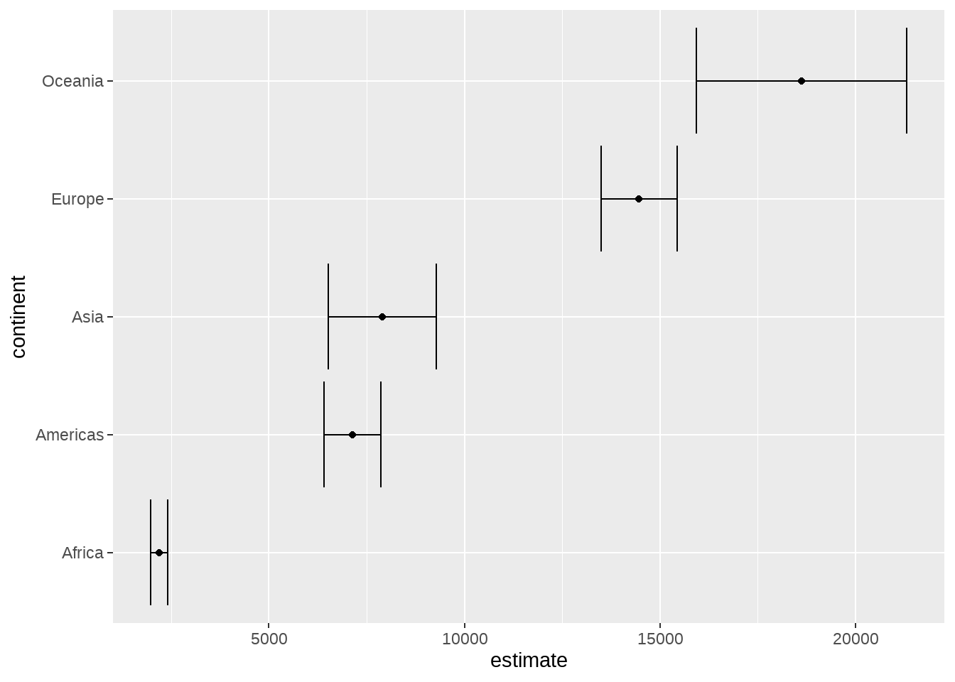
## 5 Oceania 18622.summarize()也可以生成一个list,比如下面做单样本的t检验
library(gapminder)
gapminder %>%
  group_by(continent) %>%
  summarise(test = list(t.test(gdpPercap))) %>%

  mutate(tidied = purrr::map(test, broom::tidy)) %>%
  unnest(tidied) %>%
  ggplot(aes(estimate, continent)) +
  geom_point() +
  geom_errorbarh(aes(
    xmin = conf.low,
    xmax = conf.high
  ))
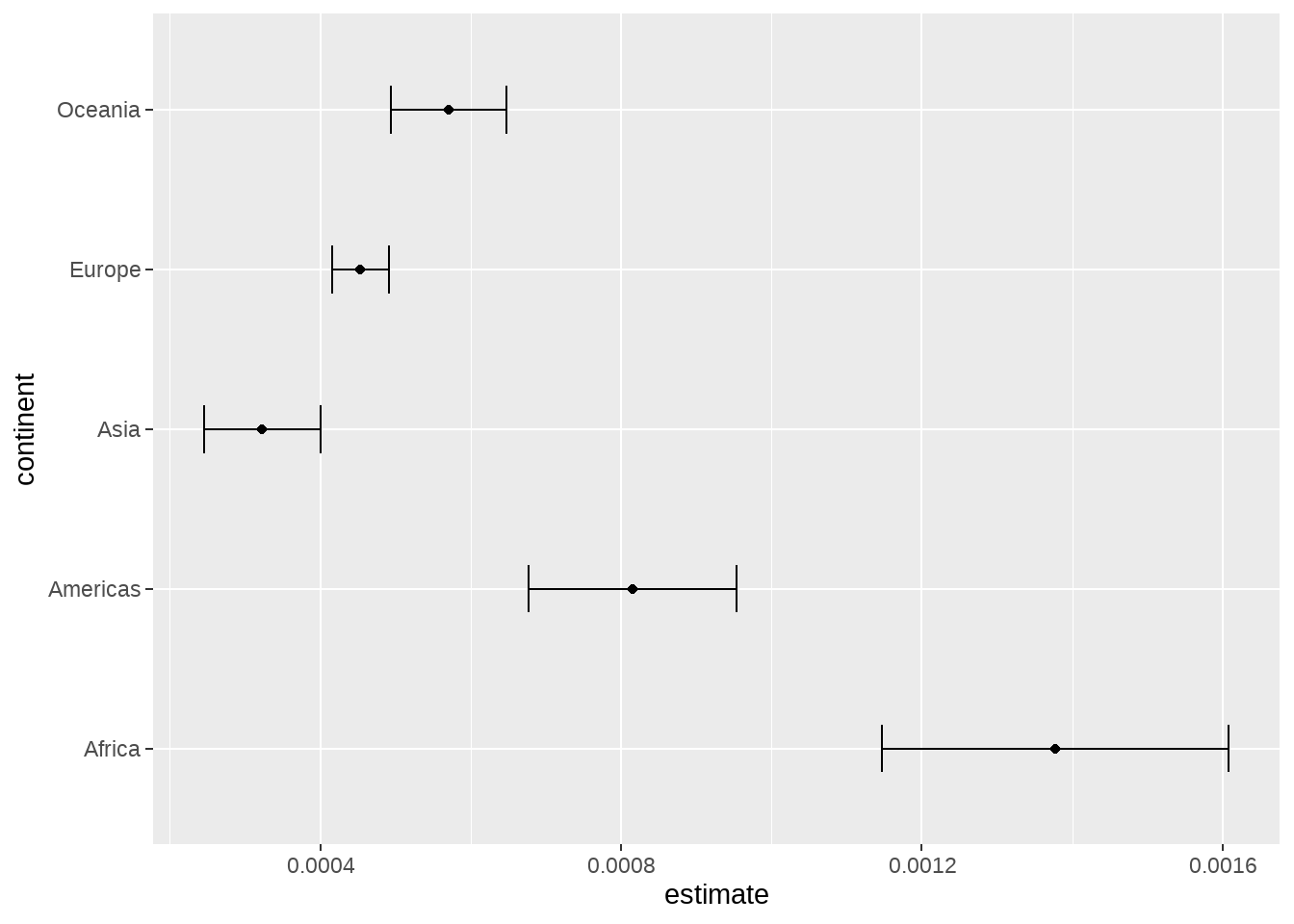
或者线性回归
gapminder %>%
  group_by(continent) %>%
  summarise(test = list(lm(lifeExp ~ gdpPercap))) %>%

  mutate(tidied = purrr::map(test, broom::tidy, conf.int = TRUE)) %>%
  unnest(tidied) %>%
  filter(term != "(Intercept)") %>%
  ggplot(aes(estimate, continent)) +
  geom_point() +
  geom_errorbarh(aes(
    xmin = conf.low,
    xmax = conf.high,
    height = .3
  ))
以下两种方法,同样完成上面的工作,具体方法会在第 37 章介绍
36.15 count() + fct_reorder() + geom_col() + coord_flip()
最好用的四件套
gapminder %>%
  distinct(continent, country) %>%
  count(continent) %>%
  ggplot(aes(x = continent, y = n)) +
  geom_col()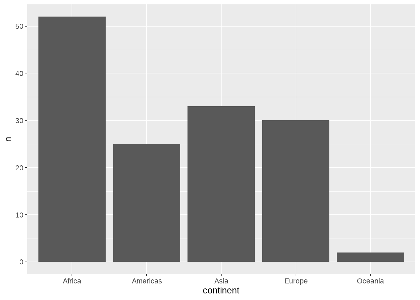
gapminder %>%
  distinct(continent, country) %>%
  count(continent) %>%
  ggplot(aes(x = fct_reorder(continent, n), y = n)) +
  geom_col() +
  coord_flip()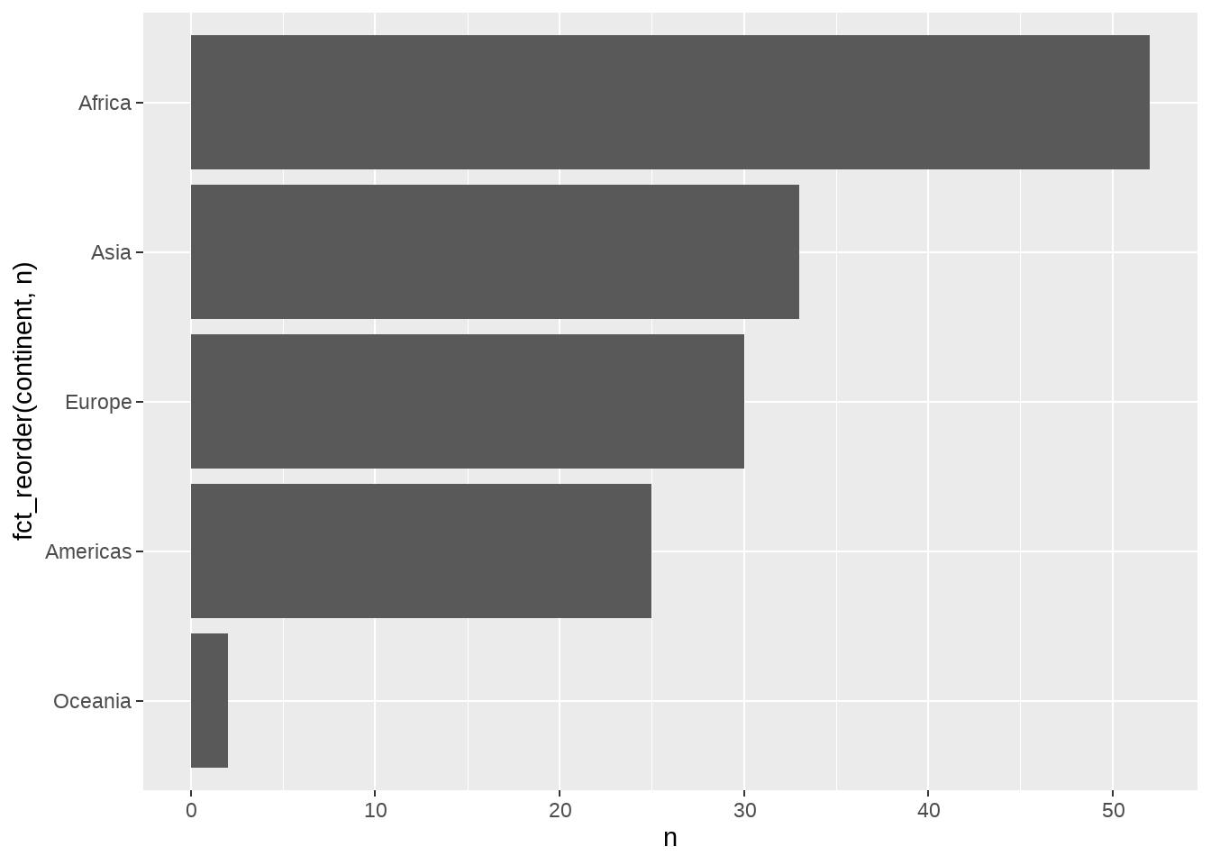
画图容易,但画出一张好图并不容易
gapminder %>%
  distinct(continent, country) %>%
  count(continent) %>%
  mutate(coll = if_else(continent == "Asia", "red", "gray")) %>%


  ggplot(aes(x = fct_reorder(continent, n), y = n)) +
  geom_text(aes(label = n), hjust = -0.25) +
  geom_col(width = 0.8, aes(fill = coll) ) +
  coord_flip() +
  theme_classic() +
  scale_fill_manual(values = c("#b3b3b3a0", "#D55E00")) +
  theme(legend.position = "none",
        axis.text = element_text(size = 11)
        ) +
  labs(title = "My title", x = "")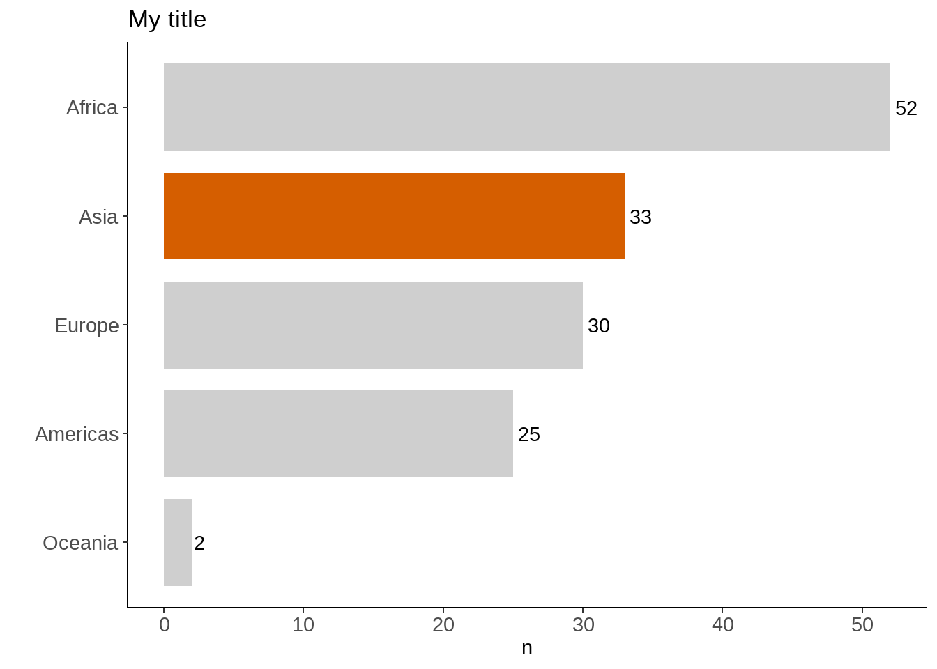
或者偷懒,将continent == "Asia"的结果直接赋值给aes(fill = ___ ), 效果与上面是一样的。
gapminder %>%
  distinct(continent, country) %>%
  count(continent) %>%


  ggplot(aes(x = fct_reorder(continent, n), y = n)) +
  geom_text(aes(label = n), hjust = -0.25) +
  geom_col(width = 0.8, aes(fill = continent == "Asia") ) +
  coord_flip() +
  theme_classic() +
  scale_fill_manual(values = c("#b3b3b3a0", "#D55E00")) +
  annotate("text", x = 3.8, y = 48, label = "this is important\ncase",
           color = "#D55E00", size = 5) +
  annotate(
    geom = "curve", x = 4.1, y = 48, xend = 4.1, yend = 35,
    curvature = .3, arrow = arrow(length = unit(2, "mm"))
  ) +
  theme(legend.position = "none",
        axis.text = element_text(size = 11)
        ) +
  labs(title = "My title", x = "")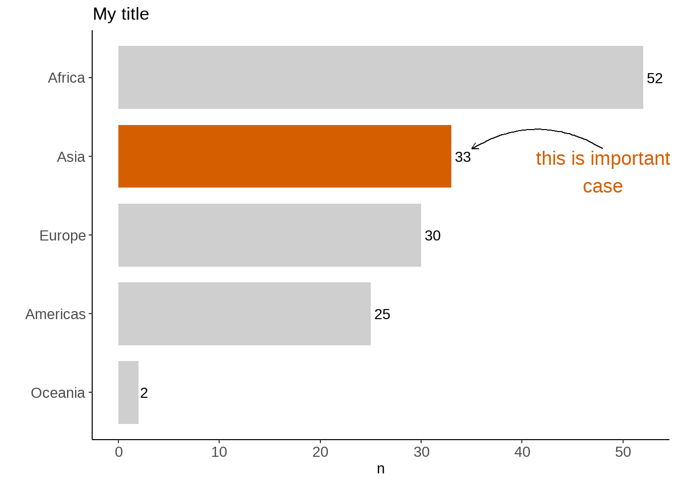
36.16 scale_x/y_log10
现实世界很多满足对数规则
- 各国人均GDP
- 各国人口
- 不同人士的收入
- 公司的营业额
gapminder %>%
  ggplot(aes(x = gdpPercap, y = lifeExp)) +
  geom_point()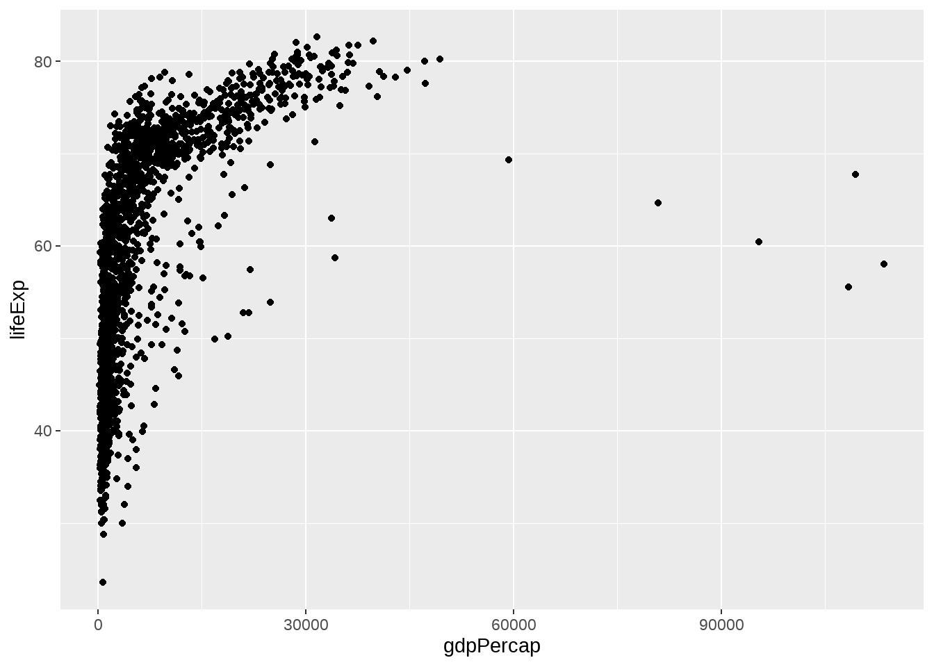
gapminder %>%
  ggplot(aes(x = gdpPercap, y = lifeExp)) +
  geom_point() +
  scale_x_log10() # A better way to log transform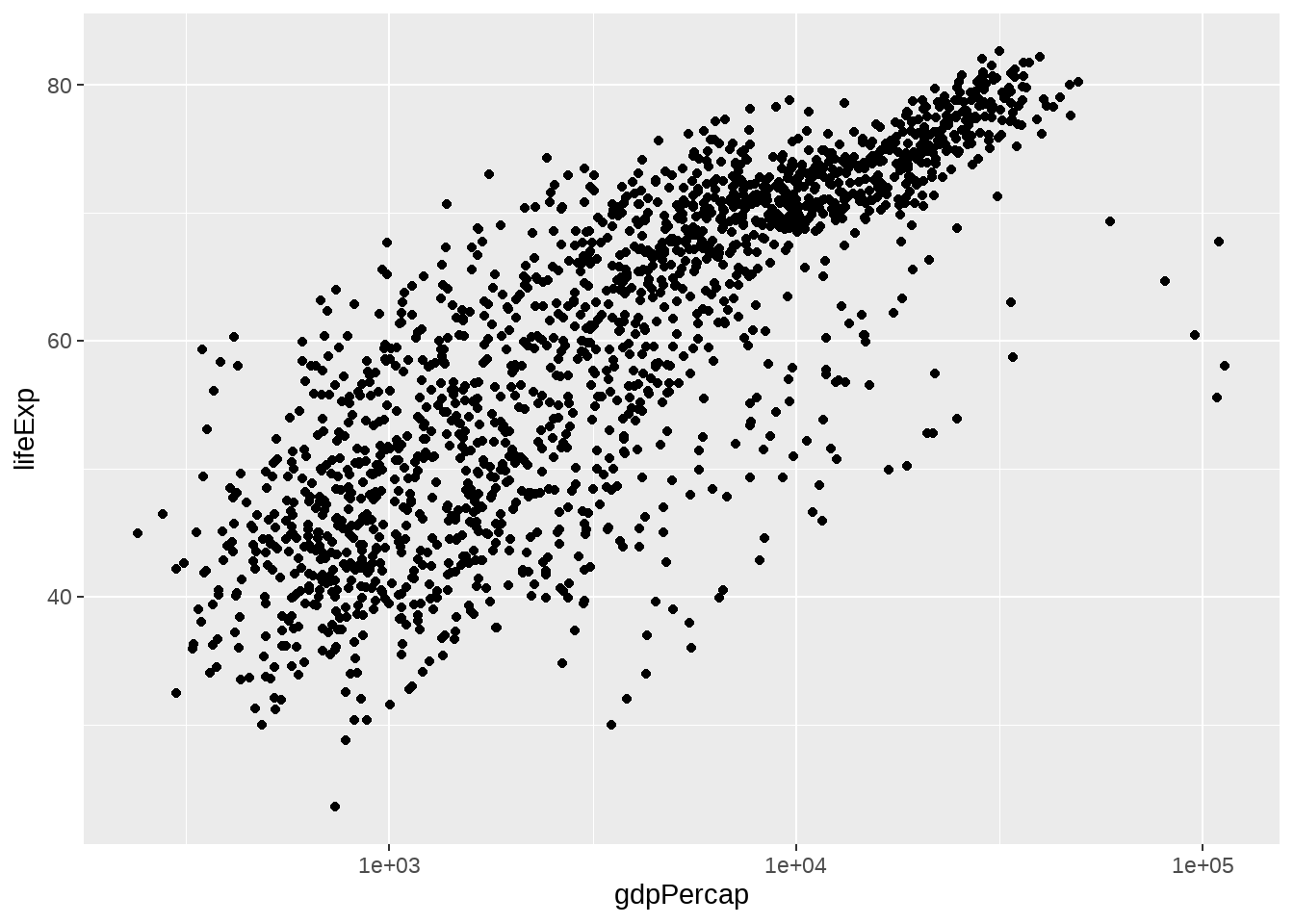
36.17 fct_lump
门诊病症的流水记录: “Stuffy nose (鼻塞)”, “Runny(流涕)”, “Fever(发热)”, “Diarrhea(腹泻)”, “Vomiting(呕吐)”, “Cough(咳嗽)”, “Sore throat(咽痛)”, “Fatigue(乏力)”, “Abdominal pain(腹痛)”, “Delusion(妄想)”, “Auditory hallucination(幻听)”, “Insomnia(失眠)”, “Anemia(贫血)”, “Hyperactivity(多动)”, “Chest pain(胸痛)”, “Chest tightness(胸闷)”,
tb <- tibble::tribble(
  ~disease, ~n,
  "Stuffy nose", 112,
  "Runny", 130,
  "Fever", 89,
  "Diarrhea", 5,
  "Vomiting", 12,
  "Cough", 102,
  "Sore throat", 98,
  "Fatigue", 15,
  "Abdominal pain", 2,
  "Delusion", 3,
  "Auditory hallucination", 6,
  "Insomnia", 1,
  "Anemia", 8,
  "Hyperactivity", 2,
  "Chest pain", 4,
  "Chest tightness", 5
)
p1 <- tb %>%
  uncount(n) %>%

  ggplot(aes(x = disease, fill = disease)) +
  geom_bar() +
  coord_flip() +
  theme(legend.position = "none")


p2 <- tb %>%
  uncount(n) %>%
  mutate(
    disease = forcats::fct_lump(disease, 5),
    disease = forcats::fct_reorder(disease, .x = disease, .fun = length)
  ) %>%
  ggplot(aes(x = disease, fill = disease)) +
  geom_bar() +
  coord_flip() +
  theme(legend.position = "none")
p1 + p2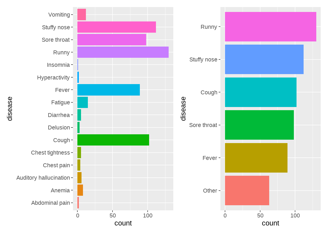
36.18 fct_reoder2
让图例的顺序与图的曲线顺序一致
dat_wide <- tibble(
  x = 1:3,
  top = c(4.5, 4, 5.5),
  middle = c(4, 4.75, 5),
  bottom = c(3.5, 3.75, 4.5)
)


dat_wide %>%
  pivot_longer(
    cols = c(top, middle, bottom),
    names_to = "region",
    values_to = "awfulness")
## # A tibble: 9 × 3
## x region awfulness
## <int> <chr> <dbl>
## 1 1 top 4.5
## 2 1 middle 4
## 3 1 bottom 3.5
## 4 2 top 4
## 5 2 middle 4.75
## 6 2 bottom 3.75
## 7 3 top 5.5
## 8 3 middle 5
## 9 3 bottom 4.5
dat <- dat_wide %>%
  pivot_longer(
    cols = c(top, middle, bottom),
    names_to = "region",
    values_to = "awfulness") %>%
  mutate(
    region_ABCD = factor(region),
    region_sane = fct_reorder2(region, x, awfulness)
  )

p_ABCD <- ggplot(dat, aes(x, awfulness, colour = region_ABCD)) +
  geom_line() + theme(legend.justification = c(1, 0.85))

p_sane <- ggplot(dat, aes(x, awfulness, colour = region_sane)) +
  geom_line() + theme(legend.justification = c(1, 0.85))

p_ABCD + p_sane +
  plot_annotation(
    title = 'Make the legend order = data order, with forcats::fct_reorder2()')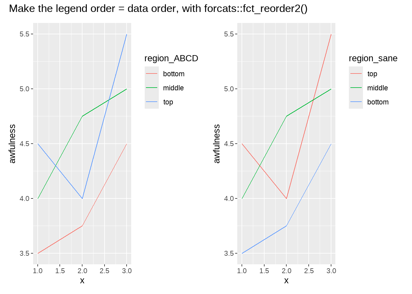
36.19 unite
dfa <- tribble(
   ~school, ~class,
  "chuansi", "01",
  "chuansi", "02",
  "shude",   "07",
  "shude",   "08",
  "huapulu", "101",
  "huapulu", "103"
)

dfa
## # A tibble: 6 × 2
## school class
## <chr> <chr>
## 1 chuansi 01
## 2 chuansi 02
## 3 shude 07
## 4 shude 08
## 5 huapulu 101
## 6 huapulu 103
df_united <- dfa %>%
   tidyr::unite(school, class, col = "school_plus_class", sep = "_", remove = FALSE)

df_united
## # A tibble: 6 × 3
## school_plus_class school class
## <chr> <chr> <chr>
## 1 chuansi_01 chuansi 01
## 2 chuansi_02 chuansi 02
## 3 shude_07 shude 07
## 4 shude_08 shude 08
## 5 huapulu_101 huapulu 101
## 6 huapulu_103 huapulu 103当然,简单的情况也可以用mutate()实现
## # A tibble: 6 × 3
##   school  class newcol
##   <chr>   <chr> <chr>
## 1 chuansi 01    chuansi_01
## 2 chuansi 02    chuansi_02
## 3 shude   07    shude_07
## 4 shude   08    shude_08
## 5 huapulu 101   huapulu_101
## 6 huapulu 103   huapulu_103
36.20 separate()
如果用mutate()来实现,语句就会比较复杂些
df_united %>%
  mutate(sch = str_split(school_plus_class, "_") %>% map_chr(1)) %>%
  mutate(cls = str_split(school_plus_class, "_") %>% map_chr(2))
## # A tibble: 6 × 5
## school_plus_class school class sch cls
## <chr> <chr> <chr> <chr> <chr>
## 1 chuansi_01 chuansi 01 chuansi 01
## 2 chuansi_02 chuansi 02 chuansi 02
## 3 shude_07 shude 07 shude 07
## 4 shude_08 shude 08 shude 08
## 5 huapulu_101 huapulu 101 huapulu 101
## 6 huapulu_103 huapulu 103 huapulu 103如果每行不是都恰好分隔成两部分呢?就需要tidyr::extract(), 使用方法和tidyr::separate()类似
dfb <- tribble(
   ~school_class,
  "chuansi_01",
  "chuansi_02_03",
  "shude_07_0",
  "shude_08_0",
  "huapulu_101_u",
  "huapulu_103__p"
)
dfb
## # A tibble: 6 × 1
## school_class
## <chr>
## 1 chuansi_01
## 2 chuansi_02_03
## 3 shude_07_0
## 4 shude_08_0
## 5 huapulu_101_u
## 6 huapulu_103__p36.21 extract()
有时候分隔符搞不定的,可以用正则表达式,将捕获的每组弄成一列
## # A tibble: 4 × 1
##   x
##   <chr>
## 1 1-12week
## 2 1-10wk
## 3 5-12w
## 4 01-05weeks## # A tibble: 4 × 4
## x start end letter
## <chr> <chr> <chr> <chr>
## 1 1-12week 1 12 week
## 2 1-10wk 1 10 wk
## 3 5-12w 5 12 w
## 4 01-05weeks 01 05 weeks36.22 crossing()
先看看效果
## # A tibble: 8 × 3
##   x     y         z
##   <chr> <chr> <int>
## 1 F     a         1
## 2 F     a         2
## 3 F     b         1
## 4 F     b         2
## 5 M     a         1
## 6 M     a         2
## 7 M     b         1
## 8 M b 2这个函数在数据模拟的时候很方便,
tidyr::crossing(trials = 1:10, m = 1:5) %>%
  group_by(trials) %>%
  mutate(
    guess = sample.int(5, n()),
    result = m == guess
  ) %>%
  summarise(score = sum(result) / n())
## # A tibble: 10 × 2
## trials score
## <int> <dbl>
## 1 1 0.4
## 2 2 0.2
## 3 3 0.2
## 4 4 0.2
## 5 5 0
## 6 6 0.2
## 7 7 0.2
## 8 8 0.2
## 9 9 0.2
## 10 10 0再来一个例子
sim <- tribble(
  ~f, ~params,
  "rbinom", list(size = 1, prob = 0.5, n = 10)
)
sim %>%
  mutate(sim = invoke_map(f, params))
## # A tibble: 1 × 3
## f params sim
## <chr> <list> <list>
## 1 rbinom <named list [3]> <int [10]>
rep_sim <- sim %>%
  crossing(rep = 1:1e5) %>%
  mutate(sim = invoke_map(f, params)) %>%
  unnest(sim) %>%
  group_by(rep) %>%
  summarise(mean_sim = mean(sim))

head(rep_sim)
## # A tibble: 6 × 2
## rep mean_sim
## <int> <dbl>
## 1 1 0.6
## 2 2 0.5
## 3 3 0.7
## 4 4 0.5
## 5 5 0.8
## 6 6 0.6
rep_sim %>%
  ggplot(aes(x = mean_sim)) +
  geom_histogram(binwidth = 0.05,  fill = "skyblue") +
  theme_classic()
也可用在较复杂的模拟,比如下面介绍的大数极限定理,
sim <- tribble(
  ~n_tosses, ~f, ~params,
     10, "rbinom", list(size = 1, prob = 0.5, n = 15),
     30, "rbinom", list(size = 1, prob = 0.5, n = 30),
    100, "rbinom", list(size = 1, prob = 0.5, n = 100),
   1000, "rbinom", list(size = 1, prob = 0.5, n = 1000),
  10000, "rbinom", list(size = 1, prob = 0.5, n = 1e4)
)
sim_rep <- sim %>%
  crossing(replication = 1:50) %>%
  mutate(sims = invoke_map(f, params)) %>%
  unnest(sims) %>%
  group_by(replication, n_tosses) %>%
  summarise(avg = mean(sims))
sim_rep %>%
  ggplot(aes(x = factor(n_tosses), y = avg)) +
  ggbeeswarm::geom_quasirandom(color = "lightgrey") +
  scale_y_continuous(limits = c(0, 1)) +
  geom_hline(
    yintercept = 0.5,
    color = "skyblue", lty = 1, size = 1, alpha = 3 / 4
  ) +
  ggthemes::theme_pander() +
  labs(
    title = "50 Replicates Of Mean 'Heads' As Number Of Tosses Increase",
    y = "mean",
    x = "Number Of Tosses"
  )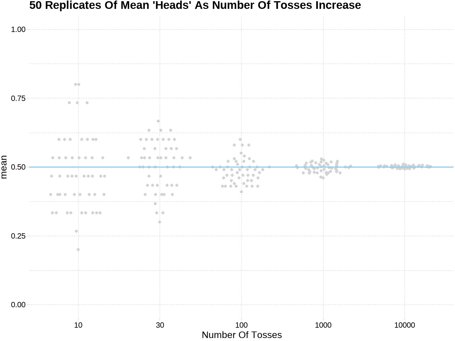
数值模拟我们会在第 48 章专门介绍。
36.23 作业
- 新建一列ratio,当sign为”positive”时,ratio等于 A除以B,当sign为”negative”时,ratio等于 B除以A
tb <- tibble::tribble(
  ~A, ~B, ~sign,
  100L, 50L, "positive",
  50L, 100L, "negative",
  100L, 50L, "positive",
  50L, 100L, "negative"
)
tb
## # A tibble: 4 × 3
## A B sign
## <int> <int> <chr>
## 1 100 50 positive
## 2 50 100 negative
## 3 100 50 positive
## 4 50 100 negative- 用
:分隔y列,并且只要前4个,构成新的数据框,并给列名c(“e1”, “e2”, “e3”, “e4”)
## # A tibble: 2 × 2
##       x y
##   <int> <chr>
## 1     1 A1:A2:A3:A4:A5:A6
## 2     2 B1:B2:B3:B4:B5:B6
最好的办法
df %>%
  separate(y, sep = ":", into = c("e1", "e2", "e3", "e4", "e5", "e6"), remove = FALSE) %>%
  select(1:6)
## # A tibble: 2 × 6
## x y e1 e2 e3 e4
## <int> <chr> <chr> <chr> <chr> <chr>
## 1 1 A1:A2:A3:A4:A5:A6 A1 A2 A3 A4
## 2 2 B1:B2:B3:B4:B5:B6 B1 B2 B3 B4其他的方法逻辑清晰, 也不错
str_split_fixed(df$y, ":", 6) %>%                   # return matrix
  # or str_split(df$y, ":", simplify = TRUE, n = 6) # return matrix
  as_tibble() %>%
  select(1:4) %>%
  set_names(c("e1", "e2", "e3", "e4"))
## # A tibble: 2 × 4
## e1 e2 e3 e4
## <chr> <chr> <chr> <chr>
## 1 A1 A2 A3 A4
## 2 B1 B2 B3 B4
df %>%
  mutate(
    new = str_split(y, pattern = ":", simplify = FALSE, n = 6) %>%
      map(., ~.x[1:4]) # return list-column: a list of vectors
  ) %>%
  unnest_wider(col = new) %>%
  set_names(c("x", "y", "e1", "e2", "e3", "e4"))
笨办法
df %>%
  mutate(
    e1 = str_split(y, pattern = ":", simplify = FALSE, n = 6) %>% map_chr(1)
  ) %>%
  mutate(
    e2 = str_split(y, pattern = ":", simplify = FALSE, n = 6) %>% map_chr(2)
  )  %>%
  mutate(
    e3 = str_split(y, pattern = ":", simplify = FALSE, n = 6) %>% map_chr(3)
  )  %>%
  mutate(
    e4 = str_split(y, pattern = ":", simplify = FALSE, n = 6) %>% map_chr(4)
  )
## # A tibble: 2 × 6
## x y e1 e2 e3 e4
## <int> <chr> <chr> <chr> <chr> <chr>
## 1 1 A1:A2:A3:A4:A5:A6 A1 A2 A3 A4
## 2 2 B1:B2:B3:B4:B5:B6 B1 B2 B3 B4