第 50 章 模拟与抽样3
我很推崇infer基于模拟的假设检验。本节课的内容是用tidyverse技术重复infer过程,让统计分析透明。
library(tidyverse)
library(infer)

penguins <- palmerpenguins::penguins %>% drop_na()

point_estimate <- penguins %>%
  specify(response = bill_length_mm) %>%
  calculate(stat = "mean")

penguins %>%
  specify(response = bill_length_mm) %>%
  hypothesize(null = "point", mu = 40) %>%
  generate(reps = 5000, type = "bootstrap") %>%
  calculate(stat = "mean") %>%
  visualize() +
  shade_p_value(obs_stat = point_estimate, direction = "two-sided")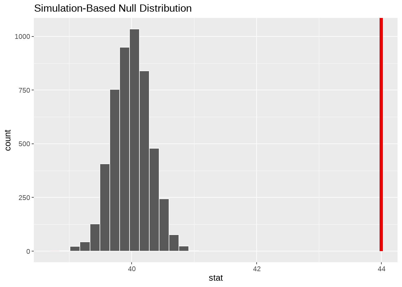
50.1 重复infer中null = "point"的抽样过程
- 零假设,bill_length_mm长度的均值是
mu = 40.
具体怎么做呢?
50.1.1 抽样
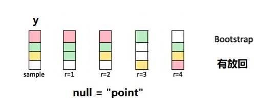
- 响应变量
y这一列,先中心化,然后加上假设条件mu - 针对调整后的这一列,有放回的抽样。
- 反复抽样
reps = 1000次
由图中可以看到,每次抽样返回的新数据框与原数据框大小相等,但因为是有放回的抽样,因此每次得到一个不同的集合,有的值可能没抽到,而有的值抽了好几次。下面以一个小的数据框为例演示
## # A tibble: 4 × 2
##       y x
##   <int> <chr>
## 1     1 a
## 2     2 a
## 3     3 b
## 4     4 b
tbl %>%
  specify(response = y) %>%
  hypothesize(null = "point", mu = 4) %>%
generate(reps = 1, type = "bootstrap") 先调整y列,然后有放回的抽样
mu <- 4
y <- tbl[[1]] - mean(tbl[[1]]) + mu
y_prime <- sample(y, size = length(y), replace = TRUE)

tbl[1] <- y_prime
tbl
也可以写成函数形式
bootstrap_once <- function(df, mu) {
  y <- df[[1]] - mean(df[[1]]) + mu
  y_prime <- sample(y, size = length(y), replace = TRUE)

  df[[1]] <- y_prime
  return(df)
}

tbl %>% bootstrap_once(mu = 4)
## # A tibble: 4 × 2
## y x
## <dbl> <chr>
## 1 5.5 a
## 2 3.5 a
## 3 4.5 b
## 4 5.5 b这个操作需要重复若干次,比如100次,即得到100个数据框,因此可以使用purrr::map()迭代
为方便灵活定义重复的次数,也可以改成函数,并且为每次返回的样本(数据框),编一个序号
bootstrap_repeat <- function(df, reps = 30, mu = mu){
  df_out <-
    purrr::map_dfr(.x = 1:reps, .f = ~ bootstrap_once(df, mu = mu)) %>%
    dplyr::mutate(replicate = rep(1:reps, each = nrow(df))) %>%
    dplyr::group_by(replicate)

  return(df_out)
}

tbl %>% bootstrap_repeat(reps = 1000, mu = 4)
## # A tibble: 4,000 × 3
## # Groups: replicate [1,000]
## y x replicate
## <dbl> <chr> <int>
## 1 4.5 a 1
## 2 4.5 a 1
## 3 2.5 b 1
## 4 2.5 b 1
## 5 2.5 a 2
## 6 4.5 a 2
## 7 3.5 b 2
## 8 2.5 b 2
## 9 4.5 a 3
## 10 3.5 a 3
## # ℹ 3,990 more rows50.1.2 计算null假设分布
计算每次抽样中,y的均值
null_dist <- tbl %>%
  bootstrap_repeat(reps = 1000, mu = 4) %>%

  group_by(replicate) %>%
  summarise(ybar = mean(y))

null_dist
## # A tibble: 1,000 × 2
## replicate ybar
## <int> <dbl>
## 1 1 5
## 2 2 3.5
## 3 3 3.5
## 4 4 4.75
## 5 5 4.25
## 6 6 5.25
## 7 7 4.5
## 8 8 3.5
## 9 9 3.75
## 10 10 4.25
## # ℹ 990 more rows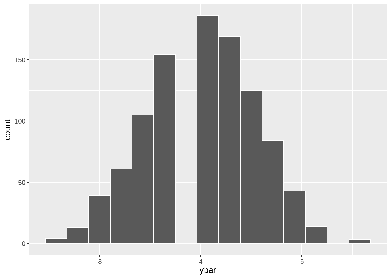
50.1.4 应用penguins
samples <- penguins %>%
select(bill_length_mm) %>%
bootstrap_repeat(reps = 5000, mu = 40)
null_dist <- samples %>%
group_by(replicate) %>%
summarise(stat = mean(bill_length_mm))
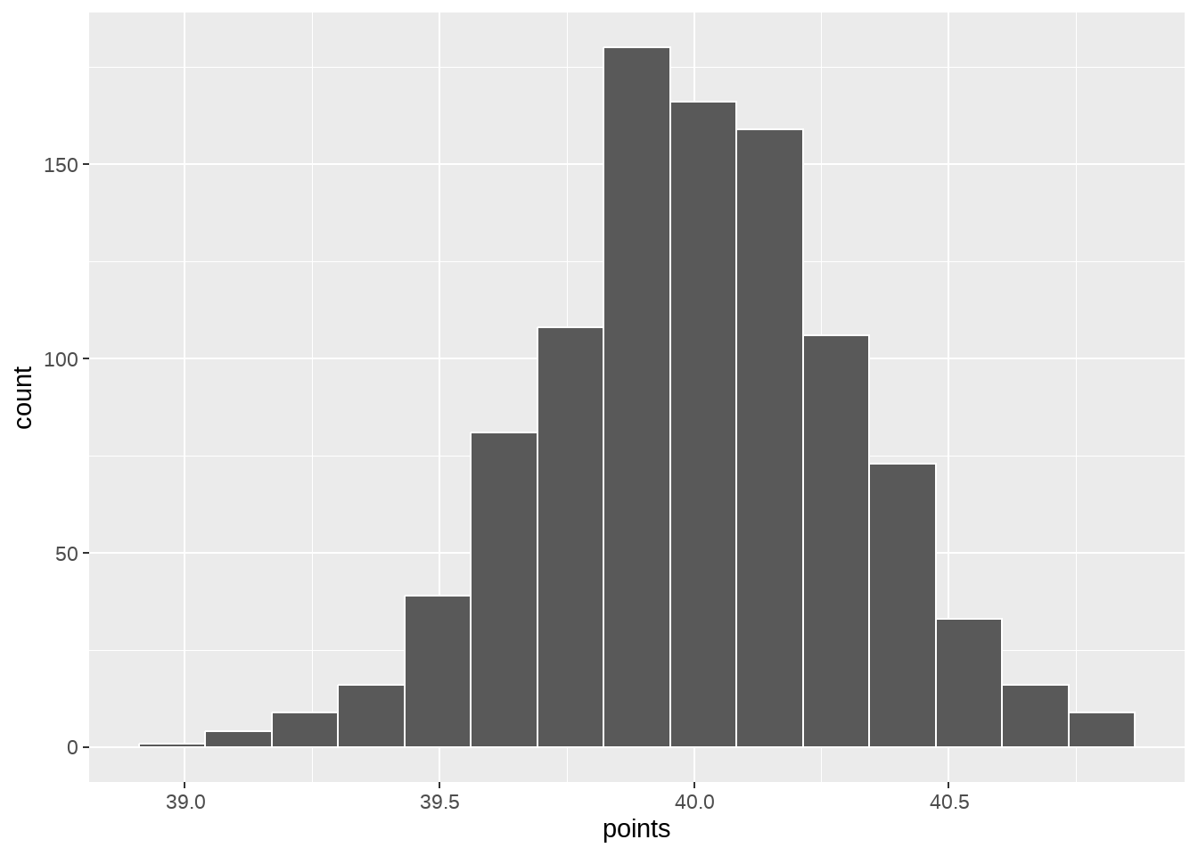
null_dist %>%
ggplot(aes(x = stat)) +
geom_histogram(bins = 15, color = "white")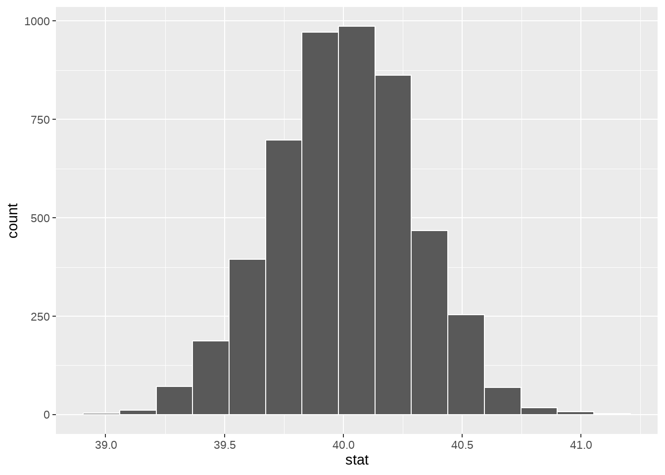
obs_point <- mean(penguins$bill_length_mm)

p_value <- sum(null_dist$stat > obs_point) / length(null_dist$stat)
p_value
## [1] 050.1.5 也可以用rowwise()写
mu <- 40

update <- penguins %>%
  mutate(
   bill_length_mm = bill_length_mm - mean(bill_length_mm) + mu
  )


null_dist <- tibble(replicate = 1:1000) %>%
  rowwise() %>%
  mutate(hand = list(sample(update$bill_length_mm, nrow(update), replace = TRUE))) %>%
  mutate(points = mean(hand)) %>%
  ungroup()

null_dist
## # A tibble: 1,000 × 3
## replicate hand points
## <int> <list> <dbl>
## 1 1 <dbl [333]> 40.0
## 2 2 <dbl [333]> 40.4
## 3 3 <dbl [333]> 40.4
## 4 4 <dbl [333]> 40.2
## 5 5 <dbl [333]> 40.1
## 6 6 <dbl [333]> 40.2
## 7 7 <dbl [333]> 40.1
## 8 8 <dbl [333]> 39.9
## 9 9 <dbl [333]> 39.8
## 10 10 <dbl [333]> 39.9
## # ℹ 990 more rows
null_dist %>%
  ggplot(aes(x = points)) +
  geom_histogram(bins = 15, color = "white")