第 74 章 抽样数据的规整与可视化
library(tidyverse)
library(tidybayes)
library(ggdist)
library(rstan)

rstan_options(auto_write = TRUE)
options(mc.cores = parallel::detectCores())在贝叶斯抽样样本量比较大,我们需要规整和可视化,就需要借助一些函数。这里简单介绍tidybayes宏包和它的姊妹宏包 ggdist,更多的技术参数见官方手册。
74.1 企鹅案例
问题简化,我们只挑选Gentoo类企鹅
## # A tibble: 119 × 8
##    species island bill_length_mm bill_depth_mm flipper_length_mm body_mass_g
##    <fct>   <fct>           <dbl>         <dbl>             <int>       <int>
##  1 Gentoo  Biscoe           46.1          13.2               211        4500
##  2 Gentoo  Biscoe           50            16.3               230        5700
##  3 Gentoo  Biscoe           48.7          14.1               210        4450
##  4 Gentoo  Biscoe           50            15.2               218        5700
##  5 Gentoo  Biscoe           47.6          14.5               215        5400
##  6 Gentoo  Biscoe           46.5          13.5               210        4550
##  7 Gentoo  Biscoe           45.4          14.6               211        4800
##  8 Gentoo  Biscoe           46.7          15.3               219        5200
##  9 Gentoo  Biscoe           43.3          13.4               209        4400
## 10 Gentoo  Biscoe           46.8          15.4               215        5150
## # ℹ 109 more rows
## # ℹ 2 more variables: sex <fct>, year <int>
先看下两个变量的关系
gentoo %>%
  ggplot(aes(x = bill_length_mm, bill_depth_mm)) +
  geom_point()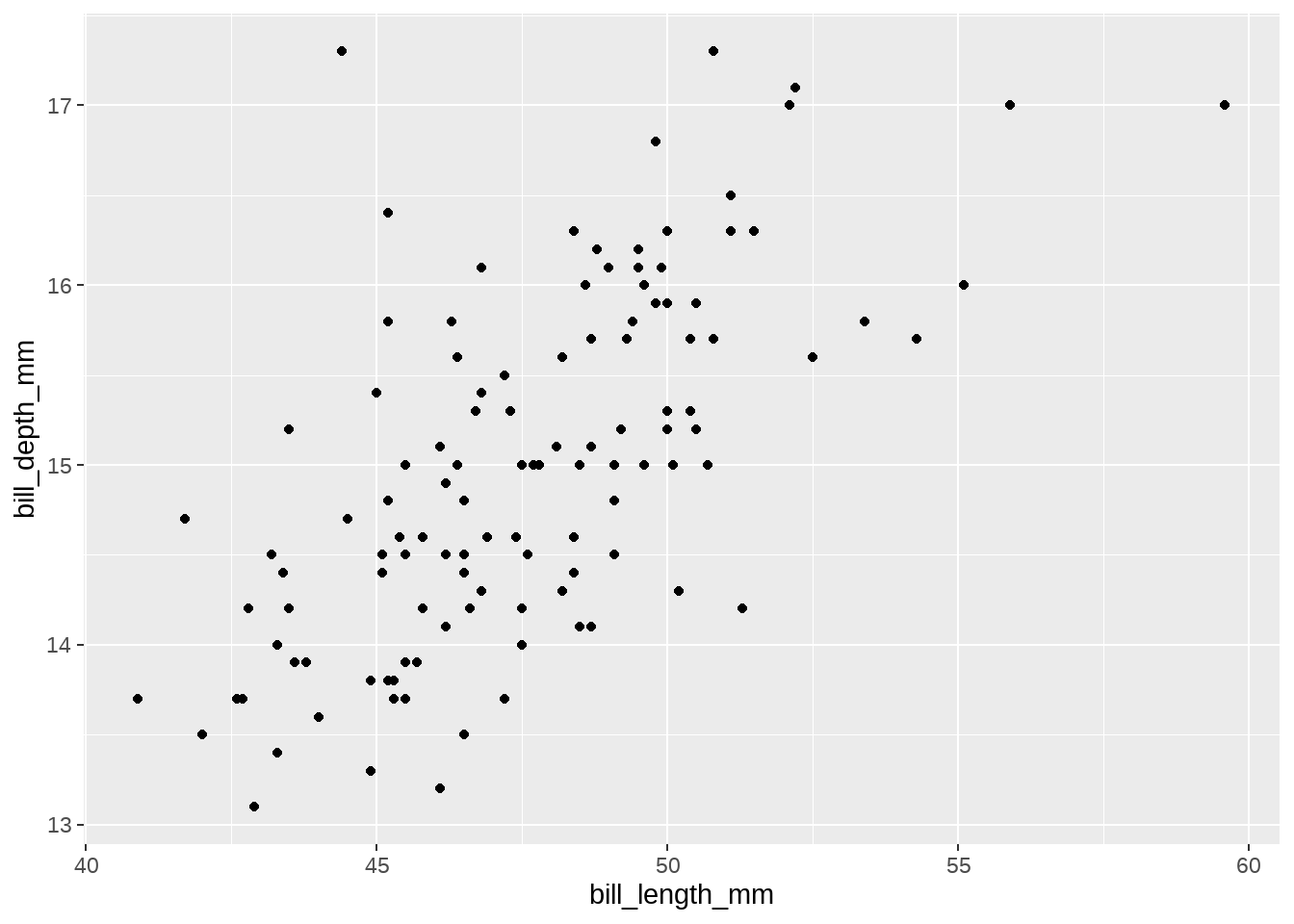
74.2 Stan模型
假设我们建立最简单的线性模型,其中预测因子bill_length_mm,被解释变量是 bill_depth_mm
\[ \begin{align} y_n &\sim \operatorname{normal}(\mu_n, \,\, \sigma)\\ \mu_n &= \alpha + \beta x_n \end{align} \]
stan_program <- "
data {
  int<lower=0> N;
  vector[N] y;
  vector[N] x;
  int<lower=0> M;
  vector[M] new_x;
}
parameters {
  real alpha;
  real beta;
  real<lower=0> sigma;
}
model {
  y ~ normal(alpha + beta * x, sigma);

  alpha  ~ normal(0, 10);
  beta   ~ normal(0, 10);
  sigma  ~ exponential(1);
}
generated quantities {
  vector[M] y_fit;
  vector[M] y_rep;
  for (n in 1:M) {
    y_fit[n] = alpha + beta * new_x[n];
    y_rep[n] = normal_rng(alpha + beta * new_x[n], sigma);
  }
}
"

library(modelr)
newdata <- gentoo %>%
  data_grid(
    bill_length_mm = seq_range(bill_length_mm, 100)
)

# or
# newdata <- data.frame(
#     bill_length_mm = seq(min(gentoo$bill_length_mm), max(gentoo$bill_length_mm), length.out = 100)
#    )


stan_data <- list(
   N = nrow(gentoo),
   x = gentoo$bill_length_mm,
   y = gentoo$bill_depth_mm,
   M = nrow(newdata),
   new_x = newdata$bill_length_mm
  )

fit <- stan(model_code = stan_program, data = stan_data)
74.3 抽样
draws <- fit %>%
  tidybayes::gather_draws(alpha, beta, sigma)
draws
## # A tibble: 12,000 × 5
## # Groups: .variable [3]
## .chain .iteration .draw .variable .value
## <int> <int> <int> <chr> <dbl>
## 1 1 1 1 alpha 3.53
## 2 1 2 2 alpha 3.10
## 3 1 3 3 alpha 3.32
## 4 1 4 4 alpha 3.21
## 5 1 5 5 alpha 3.61
## 6 1 6 6 alpha 3.87
## 7 1 7 7 alpha 2.63
## 8 1 8 8 alpha 3.99
## 9 1 9 9 alpha 3.91
## 10 1 10 10 alpha 4.76
## # ℹ 11,990 more rows74.4 统计汇总
## # A tibble: 6 × 7
##   .variable .value .lower .upper .width .point .interval
##   <chr>      <dbl>  <dbl>  <dbl>  <dbl> <chr>  <chr>
## 1 alpha      5.06   4.07   6.00    0.65 mean   qi
## 2 beta       0.209  0.189  0.229   0.65 mean   qi
## 3 sigma      0.755  0.709  0.801   0.65 mean   qi
## 4 alpha      5.06   3.33   6.76    0.89 mean   qi
## 5 beta       0.209  0.173  0.245   0.89 mean   qi
## 6 sigma      0.755  0.682  0.836   0.89 mean   qi
74.5 可视化
-
geom_slabinterval() / stat_slabinterval()family
draws %>%
  ggplot(aes(x = .value, y = .variable)) +
  ggdist::stat_interval()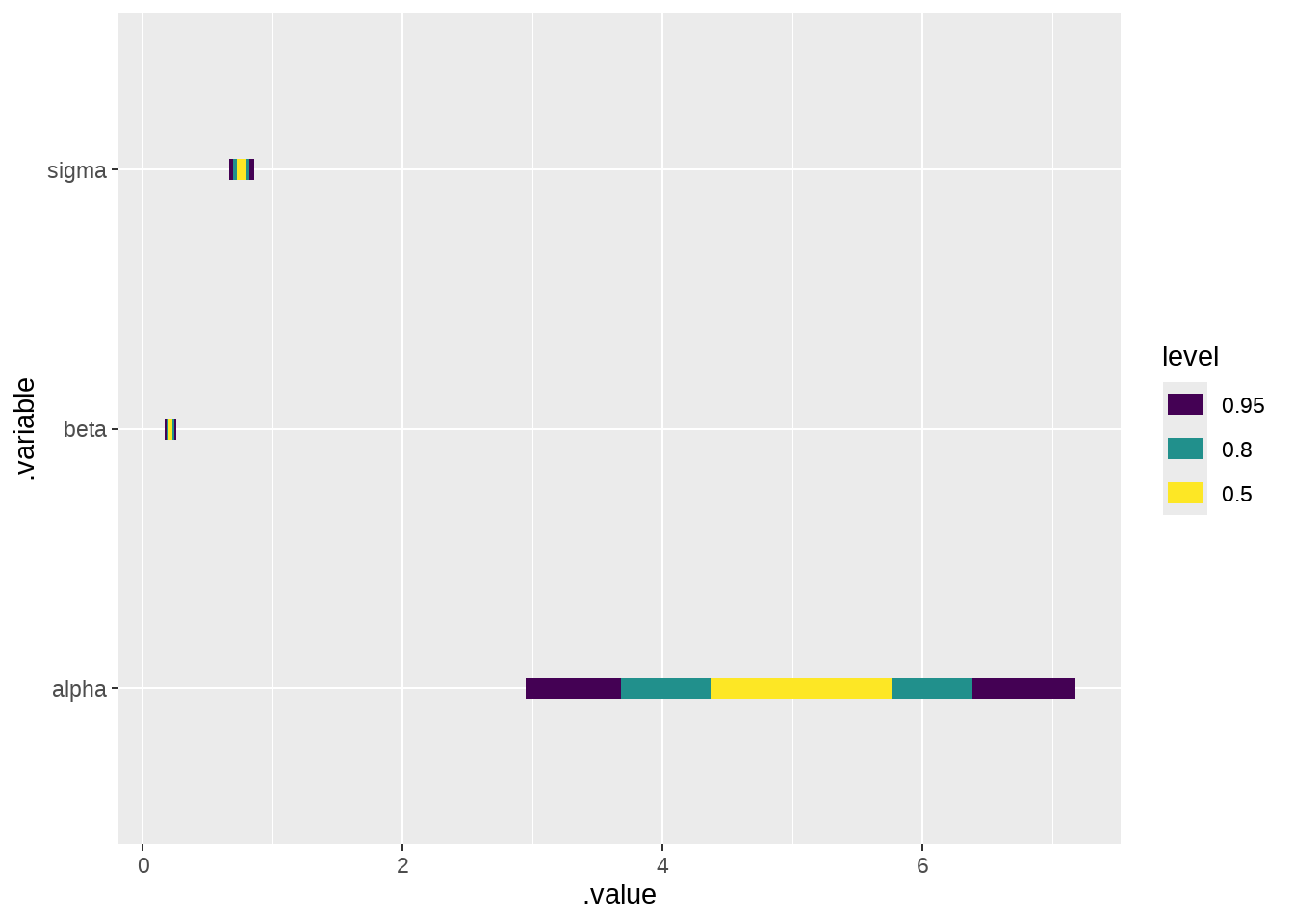
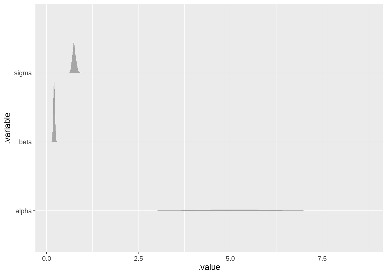
draws %>%
  ggplot(aes(x = .value, y = .variable)) +
  ggdist::stat_slabinterval()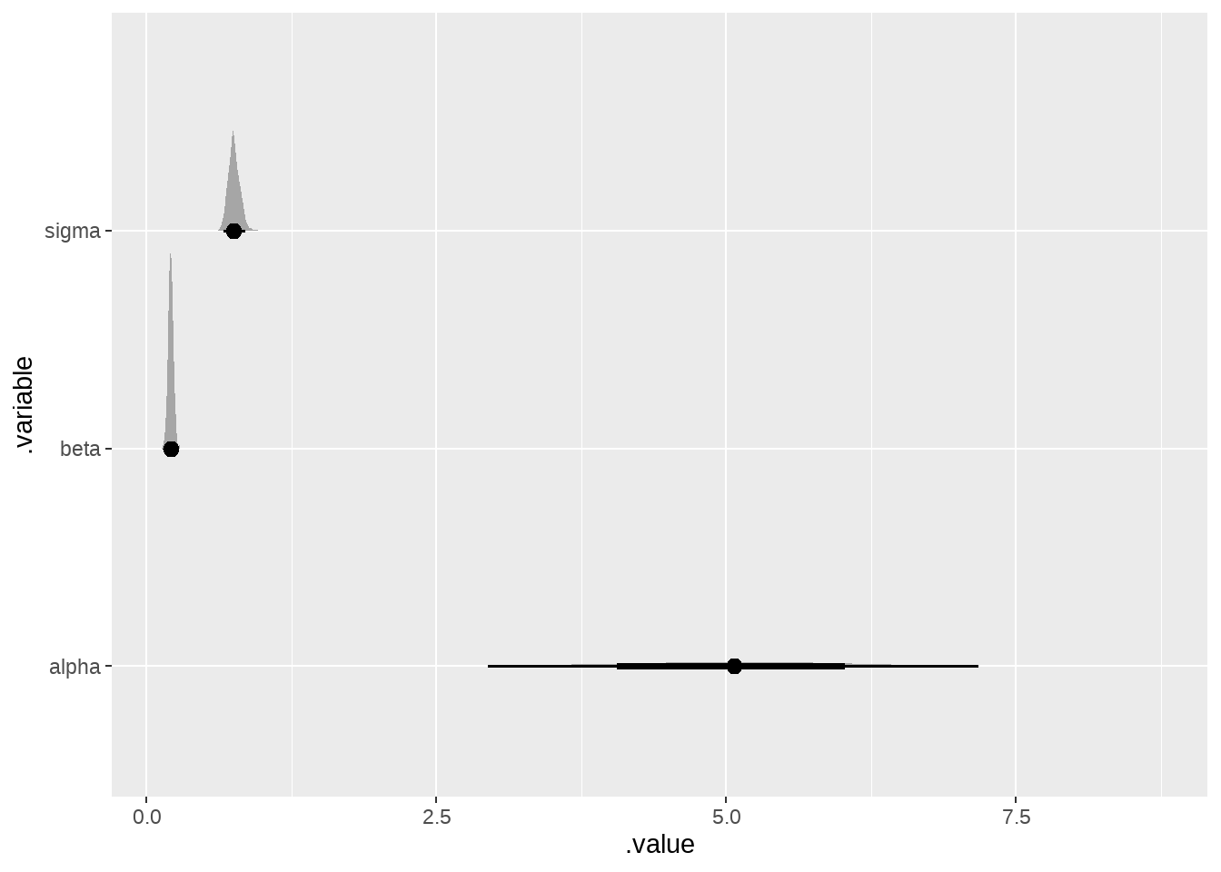
draws %>%
  filter(.variable %in% c("beta", "sigma")) %>%
  ggplot(aes(x = .value, y = .variable)) +
  ggdist::stat_slabinterval()  +
facet_grid(~ .variable, labeller = "label_both", scales = "free") 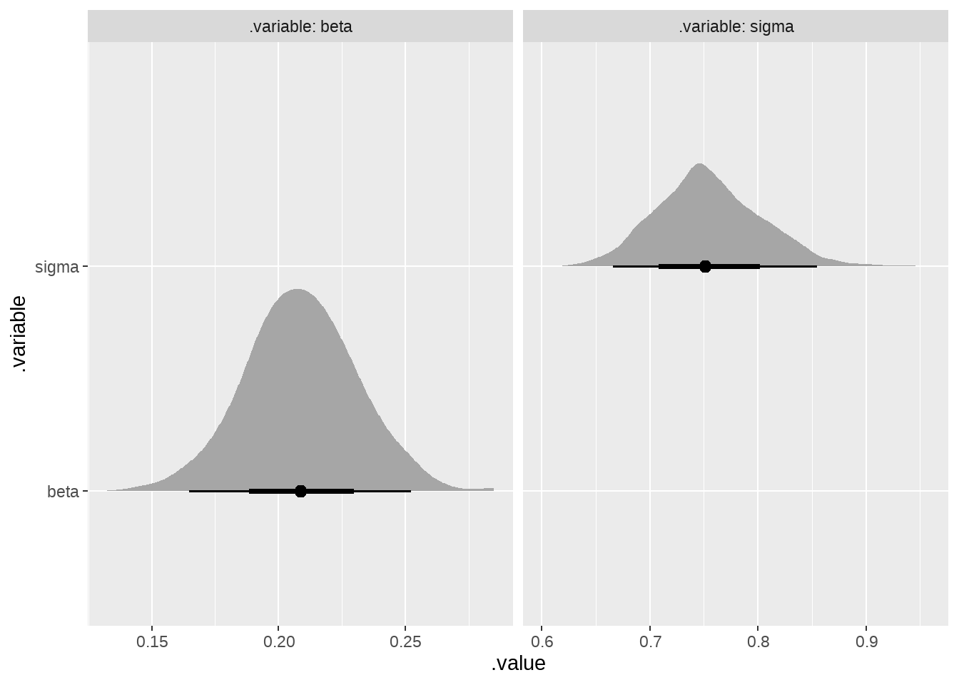
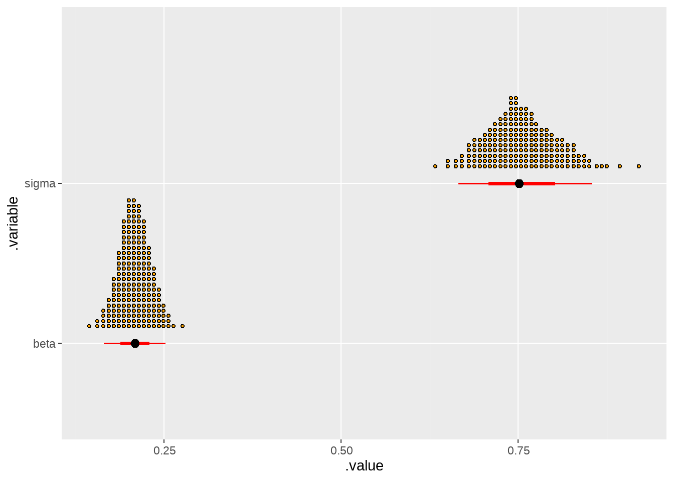
-
geom_dotsinterval() / stat_dotsinterval()family
draws %>%
  filter(.variable %in% c("beta", "sigma")) %>%
  ggplot(aes(x = .value, y = .variable)) +
  stat_dotsinterval(
    quantiles = 200,
    justification = -0.1,
    slab_color = "black",
    slab_fill = "orange",
    interval_color = "red"
) 
-
geom_lineribbon() / stat_lineribbon()family
fit %>%
  tidybayes::gather_draws(y_fit[i]) %>%
  ggdist::median_qi(.width = c(0.89)) %>%
  bind_cols(newdata) %>%

  ggplot() +
  geom_point(
    data = gentoo,
    aes(bill_length_mm, bill_depth_mm)
  ) +
  geom_lineribbon(
    aes(x = bill_length_mm, y = .value, ymin = .lower, ymax = .upper),
    alpha = 0.3,
    fill = "gray50"
  ) +
  theme_classic() +
  scale_fill_brewer(direction = -1)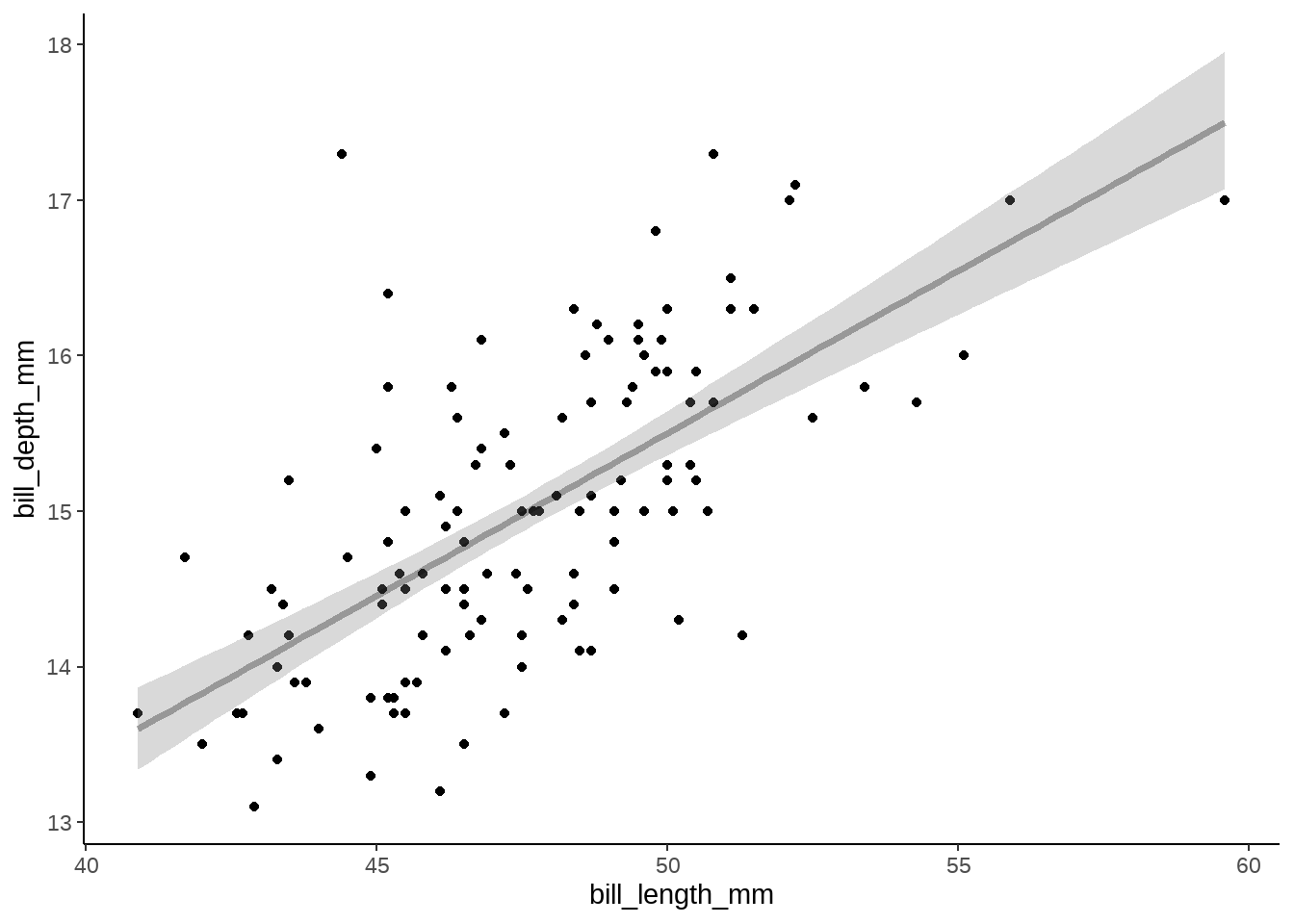
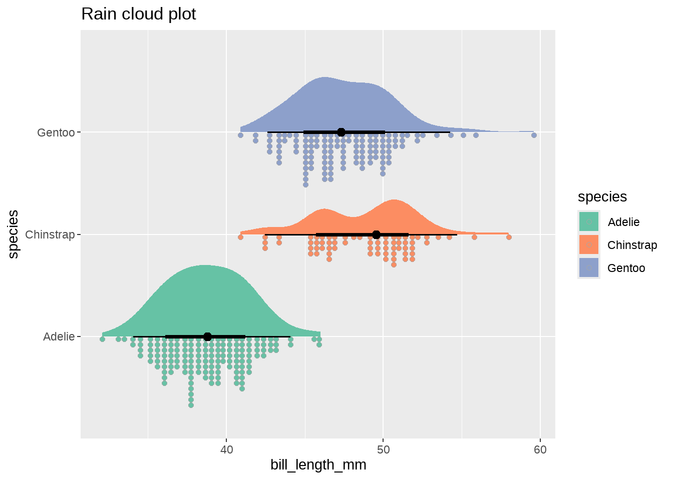
- 组合
penguins %>%
  ggplot(aes(y = species, x = bill_length_mm, fill = species)) +
  stat_slab(aes(thickness = after_stat(pdf*n)), scale = 0.7) +
  stat_dotsinterval(side = "bottom", scale = 0.7, slab_size = NA) +
  scale_fill_brewer(palette = "Set2") +
  ggtitle("Rain cloud plot")