第 73 章 贝叶斯工作流程
73.1 贝叶斯工作流程
- 数据探索和准备
- 全概率模型
- 先验预测检查,利用先验模拟响应变量
- 模型应用到模拟数据,看参数恢复情况
- 模型应用到真实数据
- 检查抽样效率和模型收敛情况
- 模型评估和后验预测检查
- 信息准则与交叉验证,以及模型选择
73.2 案例
我们用ames房屋价格,演示贝叶斯数据分析的工作流程
library(tidyverse)
library(tidybayes)
library(rstan)
rstan_options(auto_write = TRUE)
options(mc.cores = parallel::detectCores())
73.2.1 1) 数据探索和准备
rawdf <- readr::read_rds("./demo_data/ames_houseprice.rds")
rawdf
## # A tibble: 1,460 × 81
## id ms_sub_class ms_zoning lot_frontage lot_area street alley lot_shape
## <dbl> <dbl> <chr> <dbl> <dbl> <chr> <chr> <chr>
## 1 1 60 RL 65 8450 Pave <NA> Reg
## 2 2 20 RL 80 9600 Pave <NA> Reg
## 3 3 60 RL 68 11250 Pave <NA> IR1
## 4 4 70 RL 60 9550 Pave <NA> IR1
## 5 5 60 RL 84 14260 Pave <NA> IR1
## 6 6 50 RL 85 14115 Pave <NA> IR1
## 7 7 20 RL 75 10084 Pave <NA> Reg
## 8 8 60 RL NA 10382 Pave <NA> IR1
## 9 9 50 RM 51 6120 Pave <NA> Reg
## 10 10 190 RL 50 7420 Pave <NA> Reg
## # ℹ 1,450 more rows
## # ℹ 73 more variables: land_contour <chr>, utilities <chr>, lot_config <chr>,
## # land_slope <chr>, neighborhood <chr>, condition1 <chr>, condition2 <chr>,
## # bldg_type <chr>, house_style <chr>, overall_qual <dbl>, overall_cond <dbl>,
## # year_built <dbl>, year_remod_add <dbl>, roof_style <chr>, roof_matl <chr>,
## # exterior1st <chr>, exterior2nd <chr>, mas_vnr_type <chr>,
## # mas_vnr_area <dbl>, exter_qual <chr>, exter_cond <chr>, foundation <chr>, …为了简化,我们只关注房屋价格(sale_price)与房屋占地面积(lot_area)和所在地理位置(neighborhood)的关系,这里需要点准备工作
- 房屋价格与房屋占地面积这两个变量对数化处理 (why ?)
- 地理位置变量转换因子类型 (why ?)
- 房屋价格与房屋占地面积这两个变量标准化处理 (why ?)
df <- rawdf %>%
  select(sale_price, lot_area, neighborhood) %>%
  drop_na() %>%
  mutate(
    across(c(sale_price, lot_area), log),
    across(neighborhood, as.factor)
  ) %>%
  mutate(
    across(c(sale_price, lot_area), ~ (.x - mean(.x)) /sd(.x) ),
  )

head(df)
## # A tibble: 6 × 3
## sale_price lot_area neighborhood
## <dbl> <dbl> <fct>
## 1 0.560 -0.133 CollgCr
## 2 0.213 0.113 Veenker
## 3 0.734 0.420 CollgCr
## 4 -0.437 0.103 Crawfor
## 5 1.01 0.878 NoRidge
## 6 -0.384 0.858 Mitchel
df %>%
  ggplot(aes(x = lot_area, y = sale_price)) +
  geom_point(colour = "blue") +
  geom_smooth(method = lm, se = FALSE, formula = "y ~ x")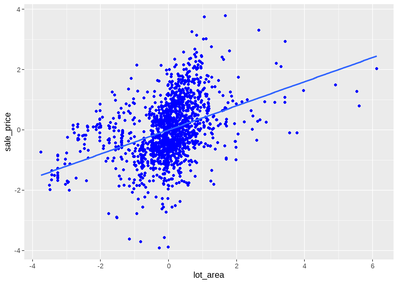
df %>%
  ggplot(aes(x = lot_area, y = sale_price)) +
  geom_point(colour = "blue") +
  geom_smooth(method = lm, se = FALSE, formula = "y ~ x", fullrange = TRUE) +
  facet_wrap(vars(neighborhood))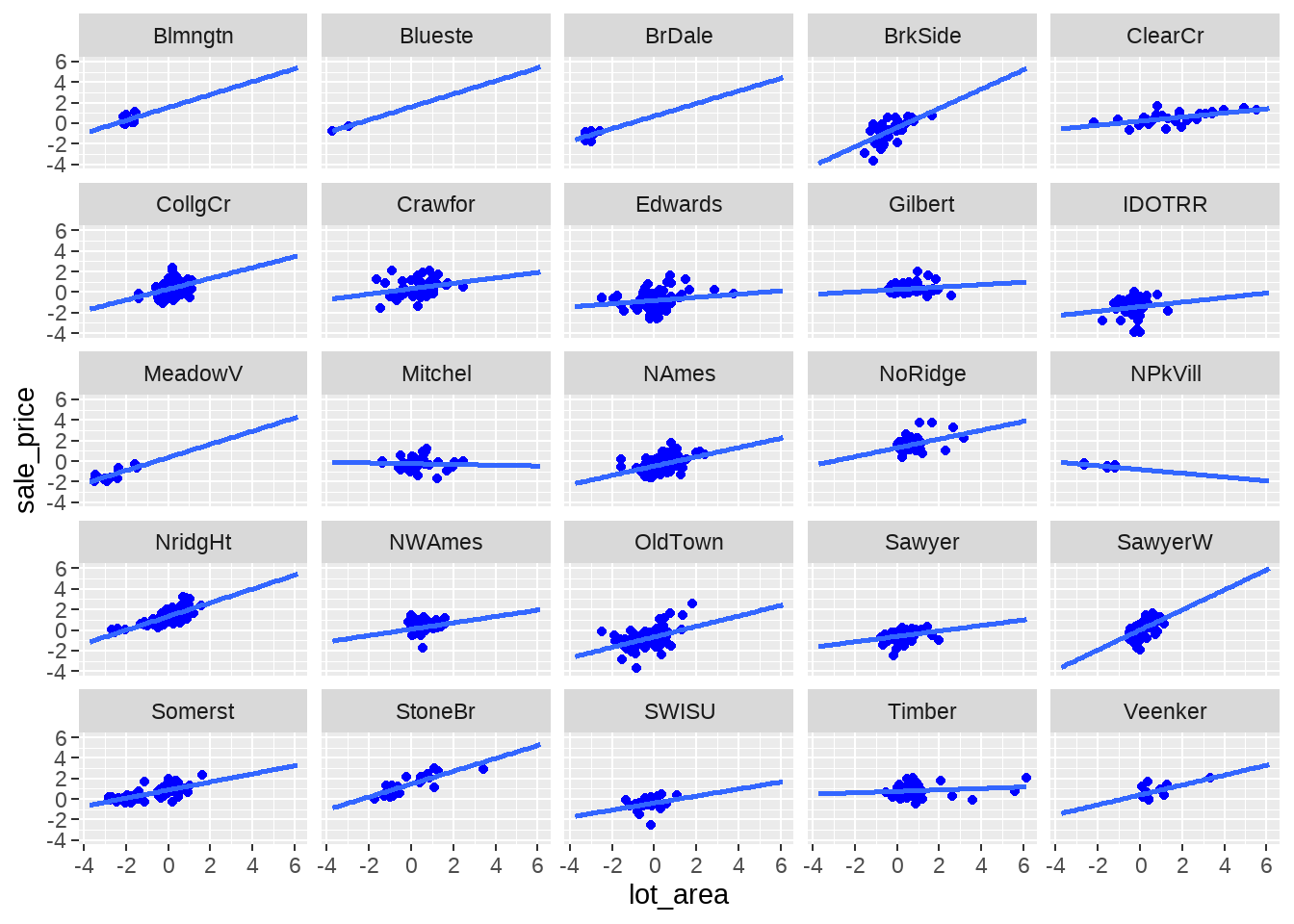
73.2.2 2) 数据模型
\[ \begin{align} y_i &\sim \operatorname{Normal}(\mu_i, \sigma) \\ \mu_i &= \alpha_{j} + \beta * x_i \\ \alpha_j & \sim \operatorname{Normal}(0, 10)\\ \beta & \sim \operatorname{Normal}(0, 10) \\ \sigma &\sim \exp(1) \end{align} \]
如果建立了这样的数学模型,可以马上写出stan代码
stan_program <- "
data {
int<lower=1> n;
int<lower=1> n_neighbour;
int<lower=1> neighbour[n];
vector[n] lot;
vector[n] price;
real alpha_sd;
real beta_sd;
int<lower = 0, upper = 1> run_estimation;
}
parameters {
vector[n_neighbour] alpha;
real beta;
real<lower=0> sigma;
}
model {
vector[n] mu;
for (i in 1:n) {
mu[i] = alpha[neighbour[i]] + beta * lot[i];
}
alpha ~ normal(0, alpha_sd);
beta ~ normal(0, beta_sd);
sigma ~ exponential(1);
if(run_estimation == 1) {
target += normal_lpdf(price | mu, sigma);
}
}
generated quantities {
vector[n] log_lik;
vector[n] y_hat;
for (j in 1:n) {
log_lik[j] = normal_lpdf(price | alpha[neighbour[j]] + beta * lot[j], sigma);
y_hat[j] = normal_rng(alpha[neighbour[j]] + beta * lot[j], sigma);
}
}
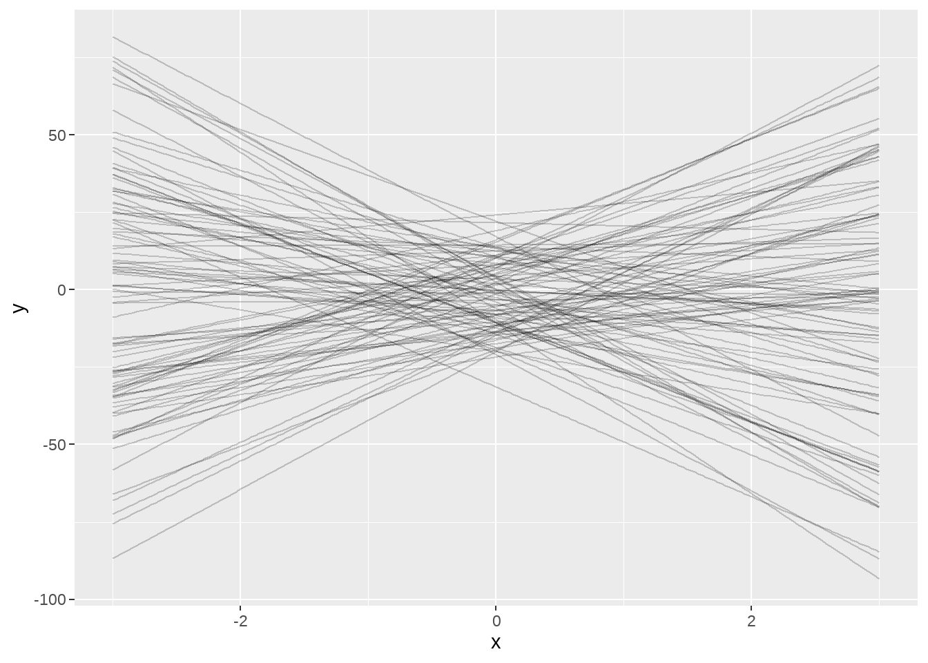
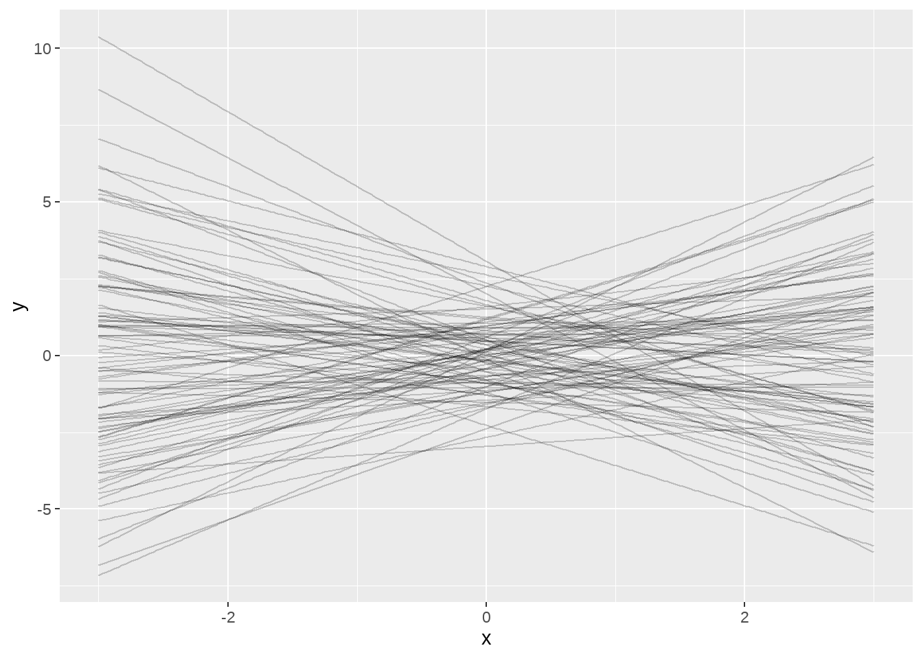
"73.2.3 3) 先验预测检查,利用先验模拟响应变量
有个问题,我们这个先验概率怎么来的呢?猜的,因为没有人知道它究竟是什么分布(如果您是这个领域的专家,就不是猜,而叫合理假设)。那到底合不合理,我们需要检验下。这里用到的技术是先验预测检验。怎么做?
- 首先,模拟先验概率分布
- 然后,通过先验和模型假定的线性关系,模拟相应的响应变量\(y_i\)(注意,不是真实的数据)
stan_data <- df %>%
  tidybayes::compose_data(
    n_neighbour    = n_distinct(neighborhood),
    neighbour      = neighborhood,
    price          = sale_price,
    lot            = lot_area,
    alpha_sd       = 10,
    beta_sd        = 10,
    run_estimation = 0
  )


model_only_prior_sd_10 <- stan(model_code = stan_program, data = stan_data,
                       chains = 1, iter = 2100, warmup = 2000)
##
## SAMPLING FOR MODEL 'anon_model' NOW (CHAIN 1).
## Chain 1:
## Chain 1: Gradient evaluation took 9.8e-05 seconds
## Chain 1: 1000 transitions using 10 leapfrog steps per transition would take 0.98 seconds.
## Chain 1: Adjust your expectations accordingly!
## Chain 1:
## Chain 1:
## Chain 1: Iteration: 1 / 2100 [ 0%] (Warmup)
## Chain 1: Iteration: 210 / 2100 [ 10%] (Warmup)
## Chain 1: Iteration: 420 / 2100 [ 20%] (Warmup)
## Chain 1: Iteration: 630 / 2100 [ 30%] (Warmup)
## Chain 1: Iteration: 840 / 2100 [ 40%] (Warmup)
## Chain 1: Iteration: 1050 / 2100 [ 50%] (Warmup)
## Chain 1: Iteration: 1260 / 2100 [ 60%] (Warmup)
## Chain 1: Iteration: 1470 / 2100 [ 70%] (Warmup)
## Chain 1: Iteration: 1680 / 2100 [ 80%] (Warmup)
## Chain 1: Iteration: 1890 / 2100 [ 90%] (Warmup)
## Chain 1: Iteration: 2001 / 2100 [ 95%] (Sampling)
## Chain 1: Iteration: 2100 / 2100 [100%] (Sampling)
## Chain 1:
## Chain 1: Elapsed Time: 3.247 seconds (Warm-up)
## Chain 1: 0.152 seconds (Sampling)
## Chain 1: 3.399 seconds (Total)
## Chain 1:
dt_wide <- model_only_prior_sd_10 %>%
  as.data.frame() %>%
  select(`alpha[5]`, beta) %>%
  rowwise() %>%
  mutate(
    set = list(tibble(
      x = seq(from = -3, to = 3, length.out = 200),
      y = `alpha[5]` + beta * x
    ))
  )


ggplot() +
  map(
    dt_wide$set,
    ~ geom_line(data = ., aes(x = x, y = y), alpha = 0.2)
  )
stan_data <- df %>%
  tidybayes::compose_data(
    n_neighbour    = n_distinct(neighborhood),
    neighbour      = neighborhood,
    price          = sale_price,
    lot            = lot_area,
    alpha_sd       = 1,
    beta_sd        = 1,
    run_estimation = 0
  )


model_only_prior_sd_1 <- stan(model_code = stan_program, data = stan_data,
                       chains = 1, iter = 2100, warmup = 2000)
##
## SAMPLING FOR MODEL 'anon_model' NOW (CHAIN 1).
## Chain 1:
## Chain 1: Gradient evaluation took 2.5e-05 seconds
## Chain 1: 1000 transitions using 10 leapfrog steps per transition would take 0.25 seconds.
## Chain 1: Adjust your expectations accordingly!
## Chain 1:
## Chain 1:
## Chain 1: Iteration: 1 / 2100 [ 0%] (Warmup)
## Chain 1: Iteration: 210 / 2100 [ 10%] (Warmup)
## Chain 1: Iteration: 420 / 2100 [ 20%] (Warmup)
## Chain 1: Iteration: 630 / 2100 [ 30%] (Warmup)
## Chain 1: Iteration: 840 / 2100 [ 40%] (Warmup)
## Chain 1: Iteration: 1050 / 2100 [ 50%] (Warmup)
## Chain 1: Iteration: 1260 / 2100 [ 60%] (Warmup)
## Chain 1: Iteration: 1470 / 2100 [ 70%] (Warmup)
## Chain 1: Iteration: 1680 / 2100 [ 80%] (Warmup)
## Chain 1: Iteration: 1890 / 2100 [ 90%] (Warmup)
## Chain 1: Iteration: 2001 / 2100 [ 95%] (Sampling)
## Chain 1: Iteration: 2100 / 2100 [100%] (Sampling)
## Chain 1:
## Chain 1: Elapsed Time: 3.18 seconds (Warm-up)
## Chain 1: 0.159 seconds (Sampling)
## Chain 1: 3.339 seconds (Total)
## Chain 1:
dt_narrow <- model_only_prior_sd_1 %>%
  as.data.frame() %>%
  select(`alpha[5]`, beta) %>%
  rowwise() %>%
  mutate(
    set = list(tibble(
      x = seq(from = -3, to = 3, length.out = 200),
      y = `alpha[5]` + beta * x
    ))
  )


ggplot() +
  map(
    dt_narrow$set,
    ~ geom_line(data = ., aes(x = x, y = y), alpha = 0.2)
  )
73.2.4 4) 模型应用到模拟数据,看参数恢复情况
df_random_draw <- model_only_prior_sd_1 %>%
  tidybayes::gather_draws(alpha[i], beta, sigma, y_hat[i], n = 1)

true_parameters <- df_random_draw %>%
  filter(.variable %in% c("alpha", "beta", "sigma")) %>%
  mutate(parameters = if_else(is.na(i), .variable, str_c(.variable, "_", i)))


y_sim <- df_random_draw %>%
  filter(.variable == "y_hat") %>%
pull(.value)模拟的数据y_sim,导入模型作为响应变量,
stan_data <- df %>%
  tidybayes::compose_data(
    n_neighbour    = n_distinct(neighborhood),
    neighbour      = neighborhood,
    price          = y_sim,      ##  这里是模拟数据
    lot            = lot_area,
    alpha_sd       = 1,
    beta_sd        = 1,
    run_estimation = 1
  )

model_on_fake_dat <- stan(model_code = stan_program, data = stan_data)
看参数恢复的如何
model_on_fake_dat %>%
  tidybayes::gather_draws(alpha[i], beta, sigma) %>%
  ungroup() %>%
  mutate(parameters = if_else(is.na(i), .variable, str_c(.variable, "_", i))) %>%

  ggplot(aes(x = .value)) +
  geom_density() +
  geom_vline(
    data = true_parameters,
    aes(xintercept = .value),
    color = "red"
    ) +
  facet_wrap(vars(parameters), ncol = 5, scales = "free")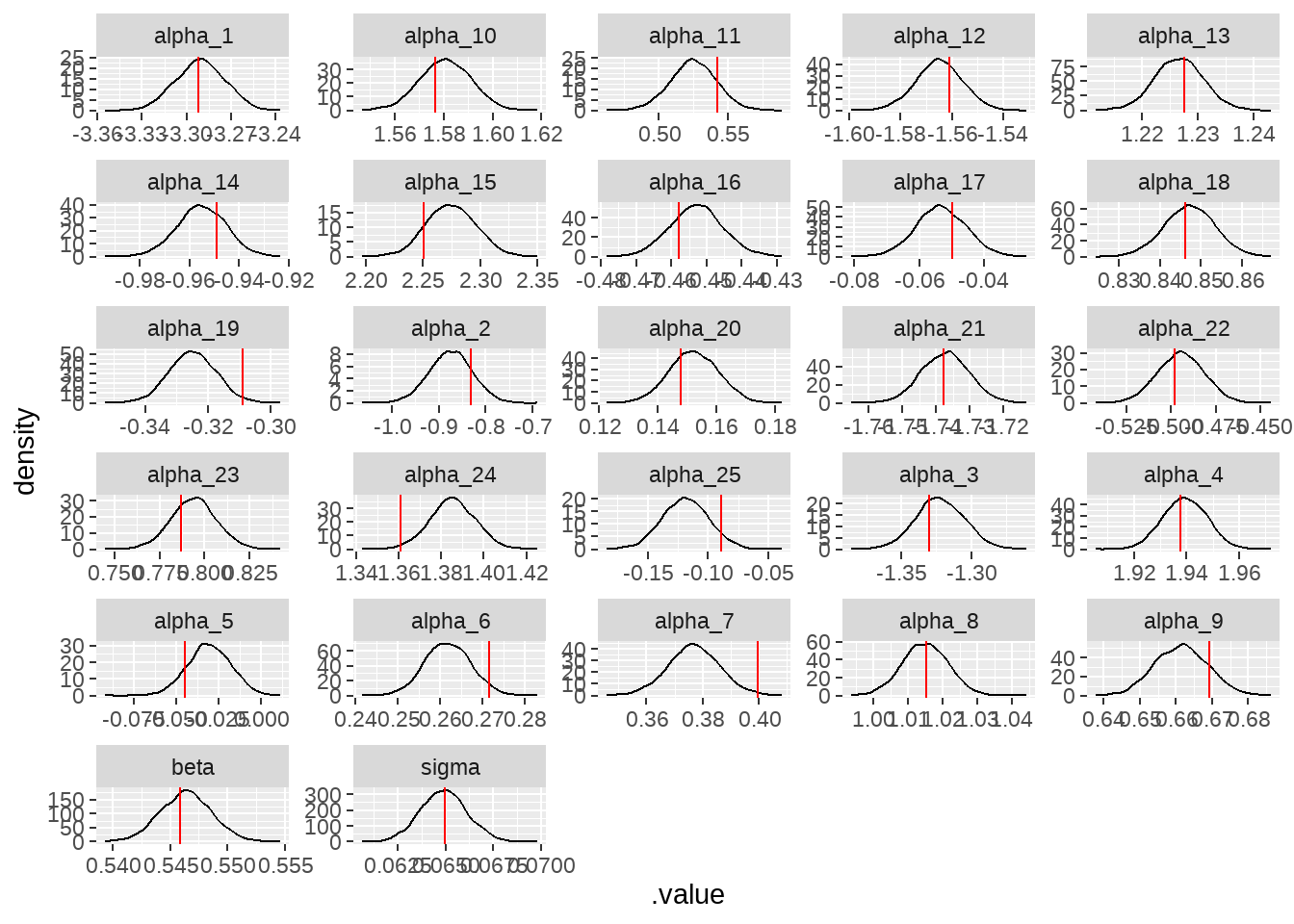
如果觉得上面的过程很麻烦,可以直接用bayesplot::mcmc_recover_hist()
posterior_alpha_beta <-
  as.matrix(model_on_fake_dat, pars = c('alpha', 'beta', 'sigma'))

bayesplot::mcmc_recover_hist(posterior_alpha_beta, true = true_parameters$.value)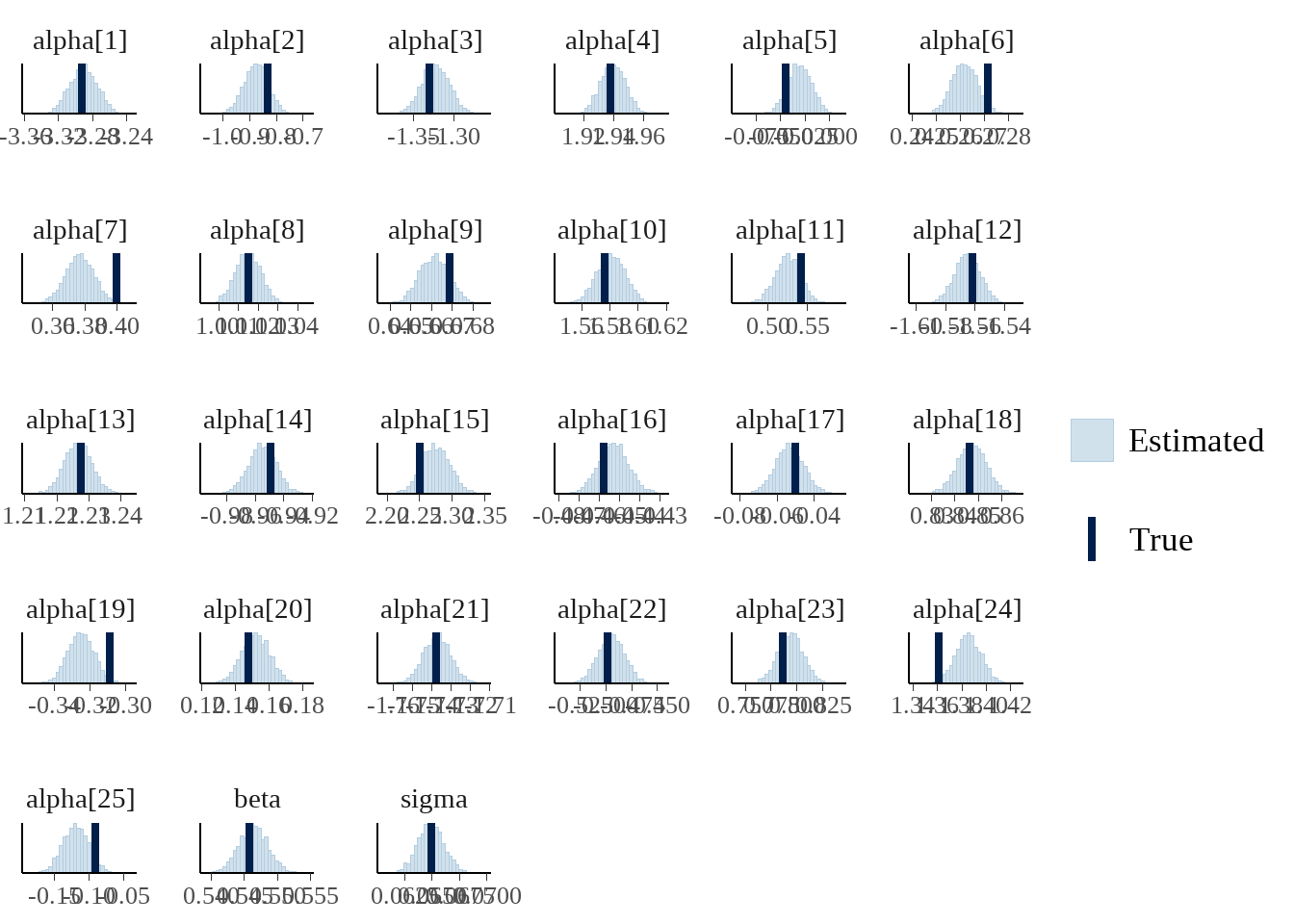
73.2.5 5) 模型应用到真实数据
应用到真实数据
stan_data <- df %>%
  tidybayes::compose_data(
    n_neighbour    = n_distinct(neighborhood),
    neighbour      = neighborhood,
    price          = sale_price,      ##  这里是真实数据
    lot            = lot_area,
    alpha_sd       = 1,
    beta_sd        = 1,
    run_estimation = 1
  )

model <- stan(model_code = stan_program, data = stan_data)
73.2.6 6) 检查抽样效率和模型收敛情况
- 检查traceplot
rstan::traceplot(model)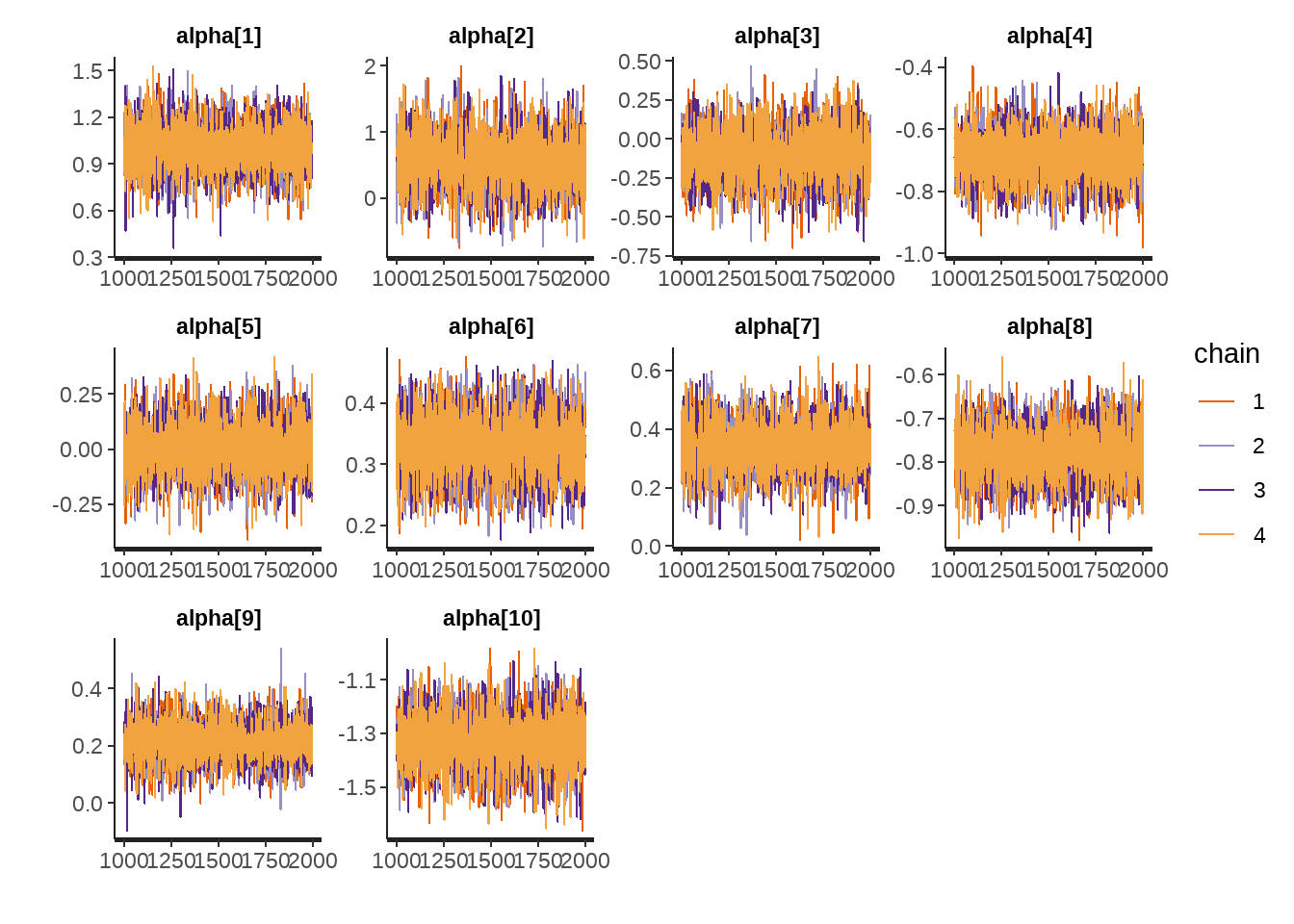
- 检查neff 和 Rhat
print(model,
  pars = c("alpha", "beta", "sigma"),
  probs = c(0.025, 0.50, 0.975),
  digits_summary = 3
)
## Inference for Stan model: anon_model.
## 4 chains, each with iter=2000; warmup=1000; thin=1;
## post-warmup draws per chain=1000, total post-warmup draws=4000.
##
## mean se_mean sd 2.5% 50% 97.5% n_eff Rhat
## alpha[1] 1.001 0.002 0.149 0.707 1.000 1.296 6805 0.999
## alpha[2] 0.568 0.005 0.403 -0.221 0.572 1.349 7243 0.999
## alpha[3] -0.100 0.002 0.164 -0.421 -0.098 0.211 6107 0.999
## alpha[4] -0.688 0.001 0.080 -0.840 -0.689 -0.535 7308 0.999
## alpha[5] 0.004 0.001 0.117 -0.223 0.002 0.239 6960 0.999
## alpha[6] 0.331 0.001 0.050 0.233 0.331 0.430 7879 0.999
## alpha[7] 0.338 0.001 0.085 0.174 0.338 0.505 6907 0.999
## alpha[8] -0.779 0.001 0.061 -0.897 -0.778 -0.662 7978 0.999
## alpha[9] 0.215 0.001 0.068 0.078 0.214 0.348 7775 0.999
## alpha[10] -1.329 0.001 0.099 -1.528 -1.328 -1.134 8280 1.000
## alpha[11] -0.409 0.002 0.154 -0.717 -0.411 -0.116 6505 1.000
## alpha[12] -0.320 0.001 0.083 -0.483 -0.321 -0.159 6473 0.999
## alpha[13] -0.439 0.000 0.040 -0.517 -0.439 -0.360 7167 0.999
## alpha[14] 1.370 0.001 0.096 1.174 1.369 1.560 7761 1.000
## alpha[15] 0.318 0.003 0.202 -0.083 0.314 0.722 6488 0.999
## alpha[16] 1.412 0.001 0.068 1.281 1.412 1.540 9192 1.000
## alpha[17] 0.100 0.001 0.073 -0.043 0.100 0.241 7046 1.000
## alpha[18] -0.685 0.001 0.057 -0.798 -0.686 -0.572 9001 1.000
## alpha[19] -0.597 0.001 0.070 -0.734 -0.597 -0.462 8282 0.999
## alpha[20] 0.120 0.001 0.079 -0.042 0.120 0.274 8366 1.000
## alpha[21] 0.870 0.001 0.066 0.744 0.872 1.000 7208 0.999
## alpha[22] 1.424 0.001 0.122 1.187 1.423 1.664 6832 0.999
## alpha[23] -0.359 0.001 0.119 -0.591 -0.360 -0.120 7653 1.000
## alpha[24] 0.505 0.001 0.098 0.312 0.506 0.698 6599 1.000
## alpha[25] 0.516 0.002 0.187 0.152 0.518 0.881 8388 0.999
## beta 0.347 0.000 0.021 0.306 0.348 0.388 3653 1.000
## sigma 0.607 0.000 0.011 0.585 0.607 0.630 7468 0.999
##
## Samples were drawn using NUTS(diag_e) at Mon Oct 28 09:59:38 2024.
## For each parameter, n_eff is a crude measure of effective sample size,
## and Rhat is the potential scale reduction factor on split chains (at
## convergence, Rhat=1).- 检查posterior sample
model %>%
  tidybayes::gather_draws(alpha[i], beta, sigma) %>%
  ungroup() %>%
  mutate(parameters = if_else(is.na(i), .variable, str_c(.variable, "_", i))) %>%

  ggplot(aes(x = .value, y = parameters)) +
  ggdist::stat_halfeye()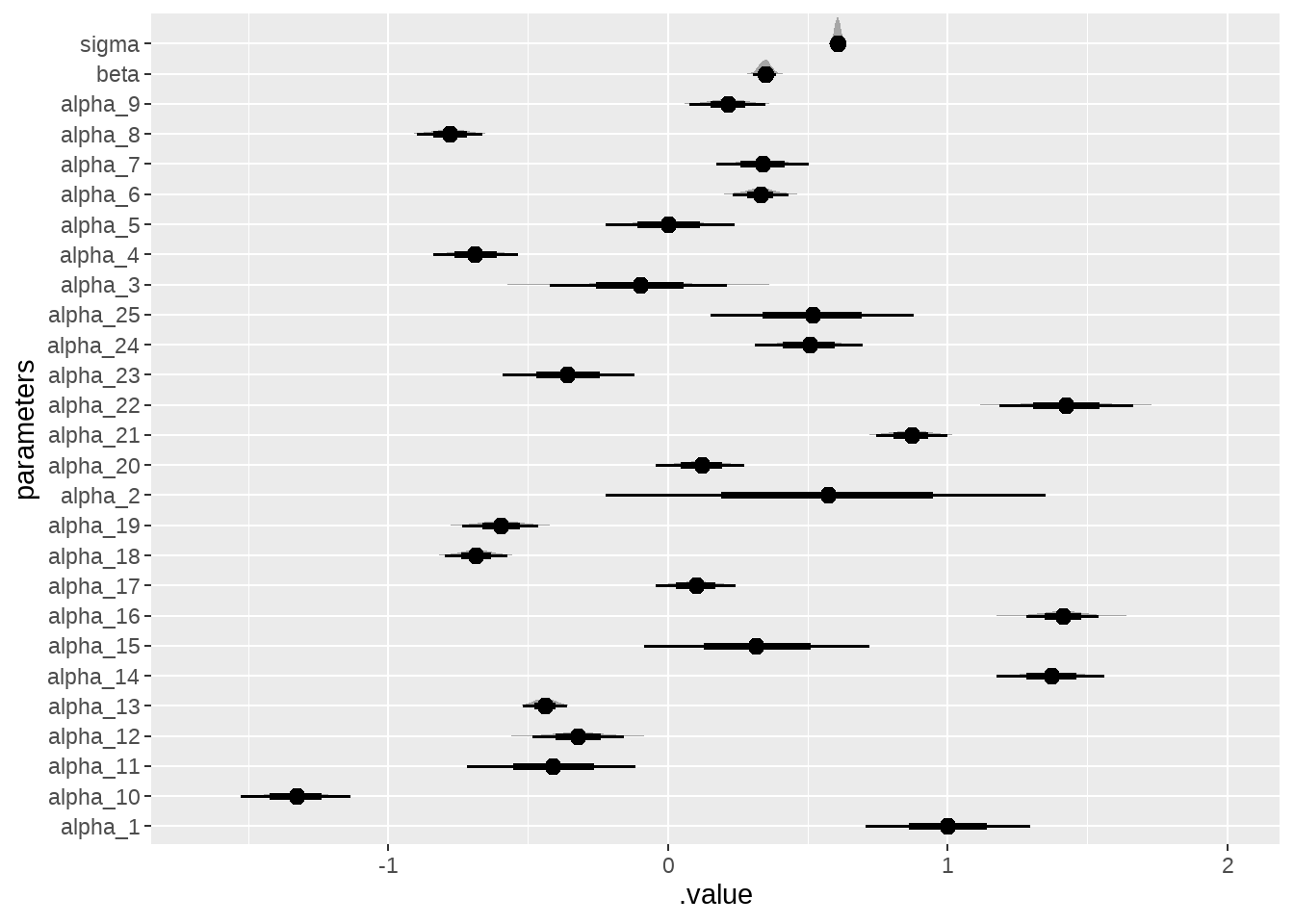
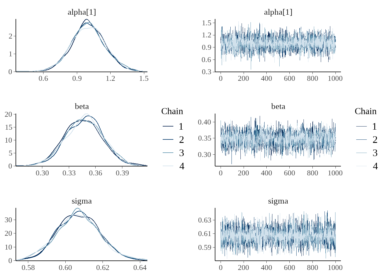
事实上,bayesplot宏包很强大也很好用
bayesplot::mcmc_combo(
  as.array(model),
  combo = c("dens_overlay", "trace"),
  pars = c('alpha[1]', 'beta', 'sigma')
) 
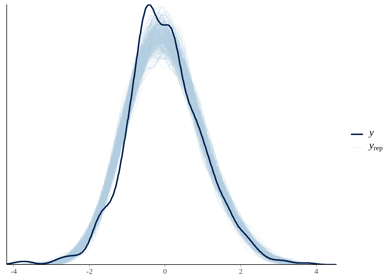
73.2.7 7) 模型评估和后验预测检查
yrep <- extract(model)[["y_hat"]]

samples <- sample(nrow(yrep), 300)
bayesplot::ppc_dens_overlay(as.vector(df$sale_price), yrep[samples, ])