第 82 章 探索性数据分析-企鹅的故事

今天讲一个关于企鹅的数据故事。这个故事来源于科考人员记录的大量企鹅体征数据，图片来源这里.

82.1 数据

82.1.1 导入数据

可通过宏包palmerpenguins::penguins获取数据，也可以读取本地penguins.csv文件， 我们采取后面一种方法：

library(tidyverse)
penguins <- read_csv("./demo_data/penguins.csv") %>%
  janitor::clean_names()

penguins %>%
  head()

## # A tibble: 6 × 8
##   species island    bill_length_mm bill_depth_mm flipper_length_mm body_mass_g
##   <chr>   <chr>              <dbl>         <dbl>             <dbl>       <dbl>
## 1 Adelie  Torgersen           39.1          18.7               181        3750
## 2 Adelie  Torgersen           39.5          17.4               186        3800
## 3 Adelie  Torgersen           40.3          18                 195        3250
## 4 Adelie  Torgersen           NA            NA                  NA          NA
## 5 Adelie  Torgersen           36.7          19.3               193        3450
## 6 Adelie  Torgersen           39.3          20.6               190        3650
## # ℹ 2 more variables: sex <chr>, year <dbl>

82.1.2 变量含义

variable	class	description
species	integer	企鹅种类 (Adelie, Gentoo, Chinstrap)
island	integer	所在岛屿 (Biscoe, Dream, Torgersen)
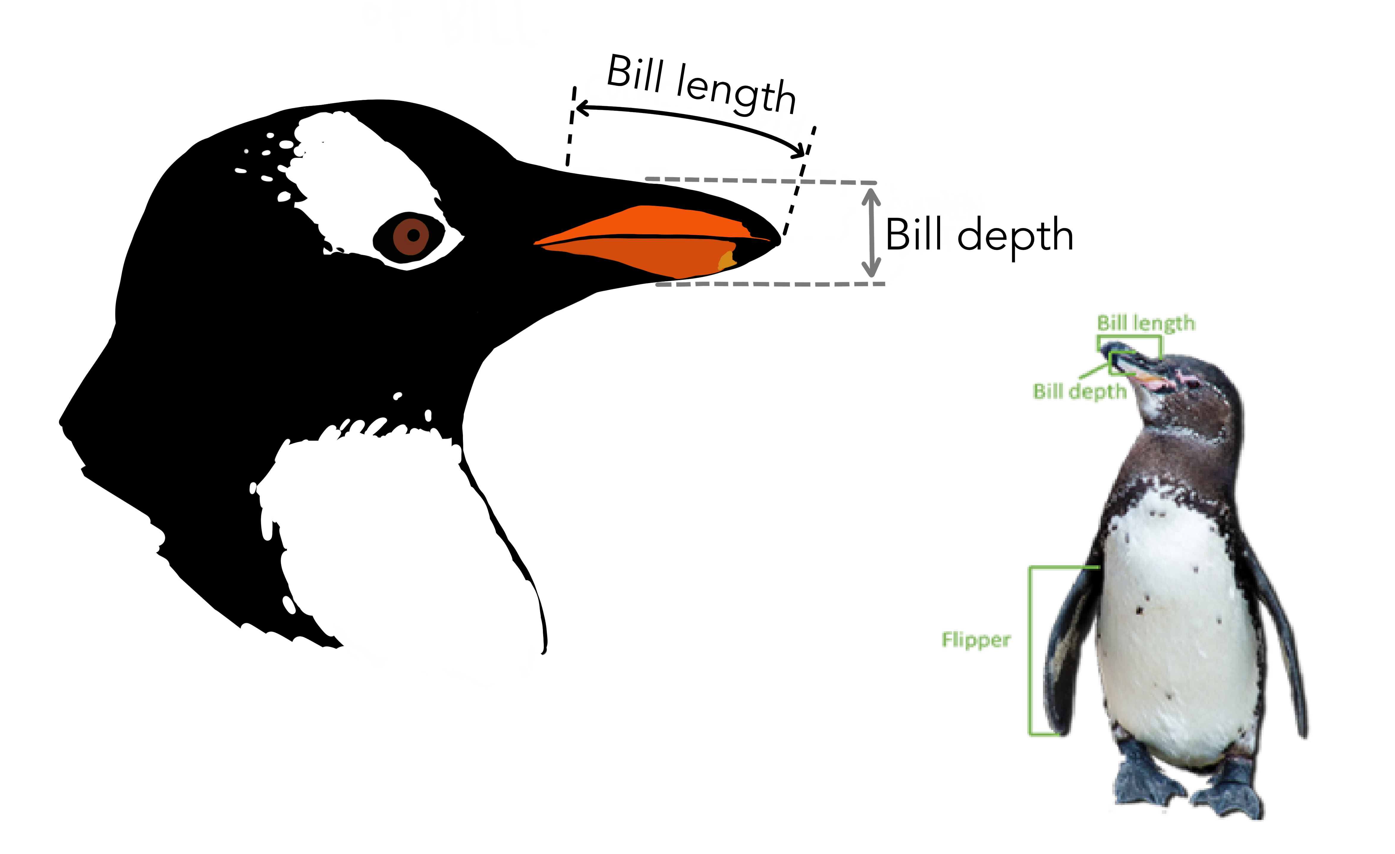
bill_length_mm	double	嘴峰长度 (单位毫米)
bill_depth_mm	double	嘴峰深度 (单位毫米)
flipper_length_mm	integer	鰭肢长度 (单位毫米)
body_mass_g	integer	体重 (单位克)
sex	integer	性别
year	integer	记录年份

82.1.3 数据清洗

检查缺失值(NA)这个很重要！

penguins %>% summarise(
  across(everything(), ~ sum(is.na(.)))
)

## # A tibble: 1 × 8
##   species island bill_length_mm bill_depth_mm flipper_length_mm body_mass_g
##     <int>  <int>          <int>         <int>             <int>       <int>
## 1       0      0              2             2                 2           2
## # ℹ 2 more variables: sex <int>, year <int>

有缺失值的地方找出来看看

penguins %>% filter_all(
  any_vars(is.na(.))
)

## # A tibble: 11 × 8
##    species island    bill_length_mm bill_depth_mm flipper_length_mm body_mass_g
##    <chr>   <chr>              <dbl>         <dbl>             <dbl>       <dbl>
##  1 Adelie  Torgersen           NA            NA                  NA          NA
##  2 Adelie  Torgersen           34.1          18.1               193        3475
##  3 Adelie  Torgersen           42            20.2               190        4250
##  4 Adelie  Torgersen           37.8          17.1               186        3300
##  5 Adelie  Torgersen           37.8          17.3               180        3700
##  6 Adelie  Dream               37.5          18.9               179        2975
##  7 Gentoo  Biscoe              44.5          14.3               216        4100
##  8 Gentoo  Biscoe              46.2          14.4               214        4650
##  9 Gentoo  Biscoe              47.3          13.8               216        4725
## 10 Gentoo  Biscoe              44.5          15.7               217        4875
## 11 Gentoo  Biscoe              NA            NA                  NA          NA
## # ℹ 2 more variables: sex <chr>, year <dbl>

发现共有11行至少有一处有缺失值，于是我们就删除这些行

penguins <- penguins %>% drop_na()
penguins

## # A tibble: 333 × 8
##    species island    bill_length_mm bill_depth_mm flipper_length_mm body_mass_g
##    <chr>   <chr>              <dbl>         <dbl>             <dbl>       <dbl>
##  1 Adelie  Torgersen           39.1          18.7               181        3750
##  2 Adelie  Torgersen           39.5          17.4               186        3800
##  3 Adelie  Torgersen           40.3          18                 195        3250
##  4 Adelie  Torgersen           36.7          19.3               193        3450
##  5 Adelie  Torgersen           39.3          20.6               190        3650
##  6 Adelie  Torgersen           38.9          17.8               181        3625
##  7 Adelie  Torgersen           39.2          19.6               195        4675
##  8 Adelie  Torgersen           41.1          17.6               182        3200
##  9 Adelie  Torgersen           38.6          21.2               191        3800
## 10 Adelie  Torgersen           34.6          21.1               198        4400
## # ℹ 323 more rows
## # ℹ 2 more variables: sex <chr>, year <dbl>

82.2 探索性分析

大家可以提出自己想探索的内容：

• 每种类型企鹅有多少只？
• 每种类型企鹅各种属性的均值和分布？
• 嘴峰长度和深度的关联？
• 体重与翅膀长度的关联？
• 嘴峰长度与嘴峰深度的比例？
• 不同种类的宝宝，体重具有显著性差异？
• 这体征中哪个因素对性别影响最大？
• …

82.2.1 每种类型企鹅有多少只

penguins %>%
  count(species, sort = T)

## # A tibble: 3 × 2
##   species       n
##   <chr>     <int>
## 1 Adelie      146
## 2 Gentoo      119
## 3 Chinstrap    68

82.2.2 每个岛屿有多少企鹅？

penguins %>%
  count(island, sort = T)

## # A tibble: 3 × 2
##   island        n
##   <chr>     <int>
## 1 Biscoe      163
## 2 Dream       123
## 3 Torgersen    47

82.2.3 每种类型企鹅各种体征属性的均值和分布

penguins %>%
  group_by(species) %>%
  summarize(across(where(is.numeric), mean, na.rm = TRUE))

## Warning: There was 1 warning in `summarize()`.
## ℹ In argument: `across(where(is.numeric), mean, na.rm = TRUE)`.
## ℹ In group 1: `species = "Adelie"`.
## Caused by warning:
## ! The `...` argument of `across()` is deprecated as of dplyr 1.1.0.
## Supply arguments directly to `.fns` through an anonymous function instead.
## 
##   # Previously
##   across(a:b, mean, na.rm = TRUE)
## 
##   # Now
##   across(a:b, \(x) mean(x, na.rm = TRUE))

## # A tibble: 3 × 6
##   species   bill_length_mm bill_depth_mm flipper_length_mm body_mass_g  year
##   <chr>              <dbl>         <dbl>             <dbl>       <dbl> <dbl>
## 1 Adelie              38.8          18.3              190.       3706. 2008.
## 2 Chinstrap           48.8          18.4              196.       3733. 2008.
## 3 Gentoo              47.6          15.0              217.       5092. 2008.

82.2.4 每种类型企鹅的嘴峰长度的分布

penguins %>%
  ggplot(aes(x = bill_length_mm)) +
  geom_density() +
  facet_wrap(vars(species), scales = "free")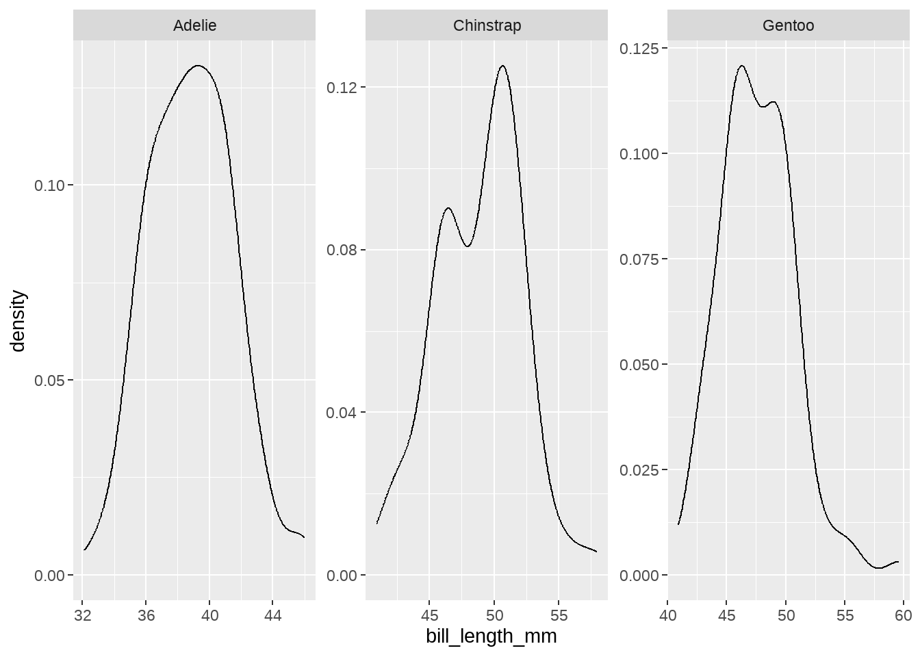

82.2.5 每种类型企鹅的嘴峰长度的分布（分性别）

penguins %>%
  ggplot(aes(x = bill_length_mm)) +
  geom_density(aes(fill = sex)) +
  facet_wrap(vars(species), scales = "free")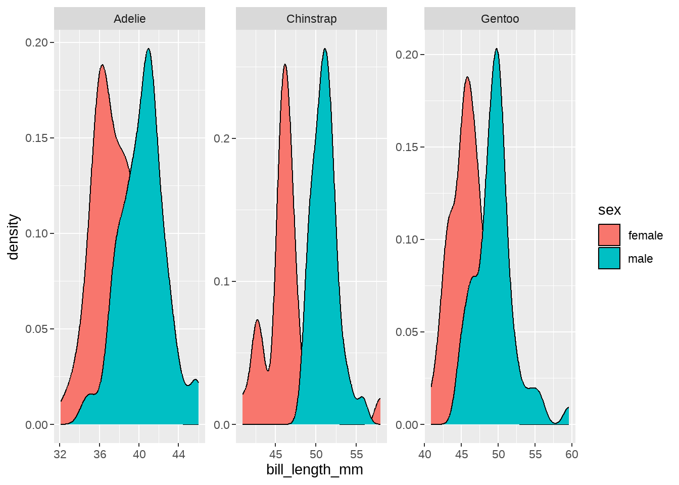

男宝宝的嘴巴要长些，哈哈。

来张更好看点的

penguins %>%
  ggplot(aes(x = bill_length_mm, fill = sex)) +
  geom_histogram(
    position = "identity",
    alpha = 0.7,
    bins = 25
  ) +
  scale_fill_manual(values = c("#66b3ff", "#8c8c8c")) +
  ylab("number of penguins") +
  xlab("length (mm)") +
  theme_minimal() +
  theme(
    legend.position = "bottom",
    legend.text = element_text(size = 11),
    legend.title = element_blank(),
    panel.grid.minor = element_blank(),
    axis.title = element_text(color = "white", size = 10),
    plot.title = element_text(size = 20),
    plot.subtitle = element_text(size = 12, hjust = 1)
  ) +
  facet_wrap(vars(species), scales = "free")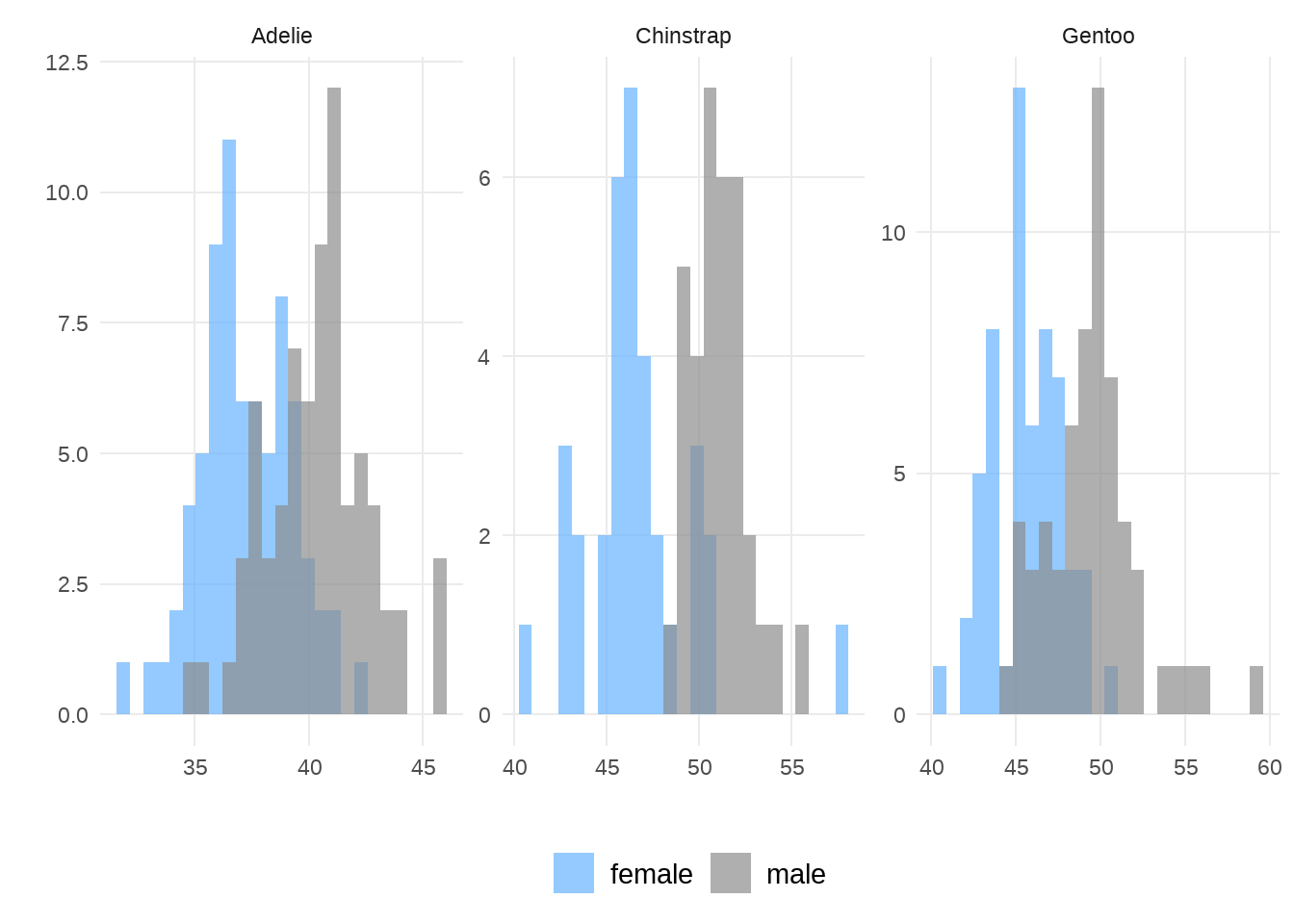

同理，可以画出其他属性的分布。当然，我更喜欢用山峦图来呈现不同分组的分布，因为竖直方向可以更方便比较

library(ggridges)

## Warning: package 'ggridges' was built under R version 4.2.2

penguins %>%
  ggplot(aes(x = bill_length_mm, y = species, fill = species)) +
  ggridges::geom_density_ridges()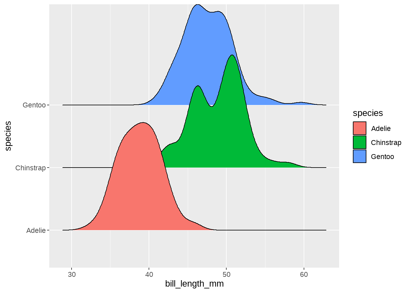

## Picking joint bandwidth of 1.08

同样，我们也用颜色区分下性别，这样不同种类、不同性别企鹅的嘴峰长度分布一目了然

penguins %>%
  ggplot(aes(x = bill_length_mm, y = species, fill = sex)) +
  geom_density_ridges(alpha = 0.5)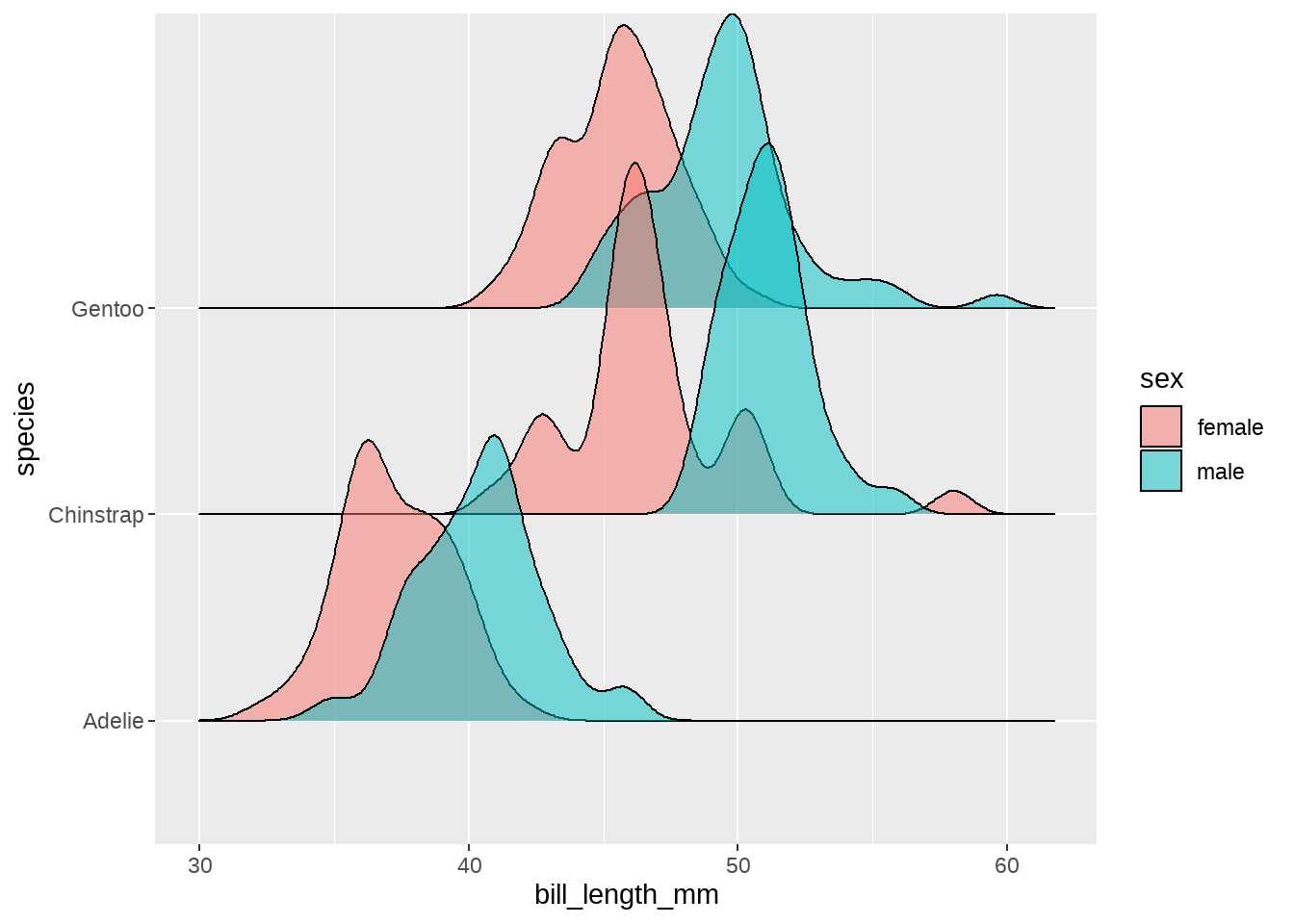

## Picking joint bandwidth of 0.717

同样的代码，类似地画个其他体征的分布，

penguins %>%
  ggplot(aes(x = bill_depth_mm, fill = species)) +
  ggridges::geom_density_ridges(aes(y = species))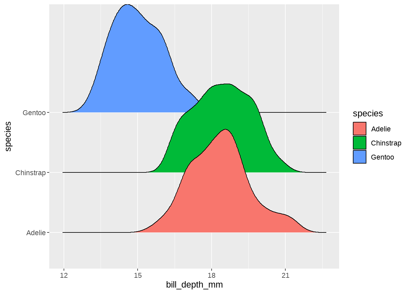

## Picking joint bandwidth of 0.384

penguins %>%
  ggplot(aes(x = bill_depth_mm, fill = sex)) +
  ggridges::geom_density_ridges(aes(y = species))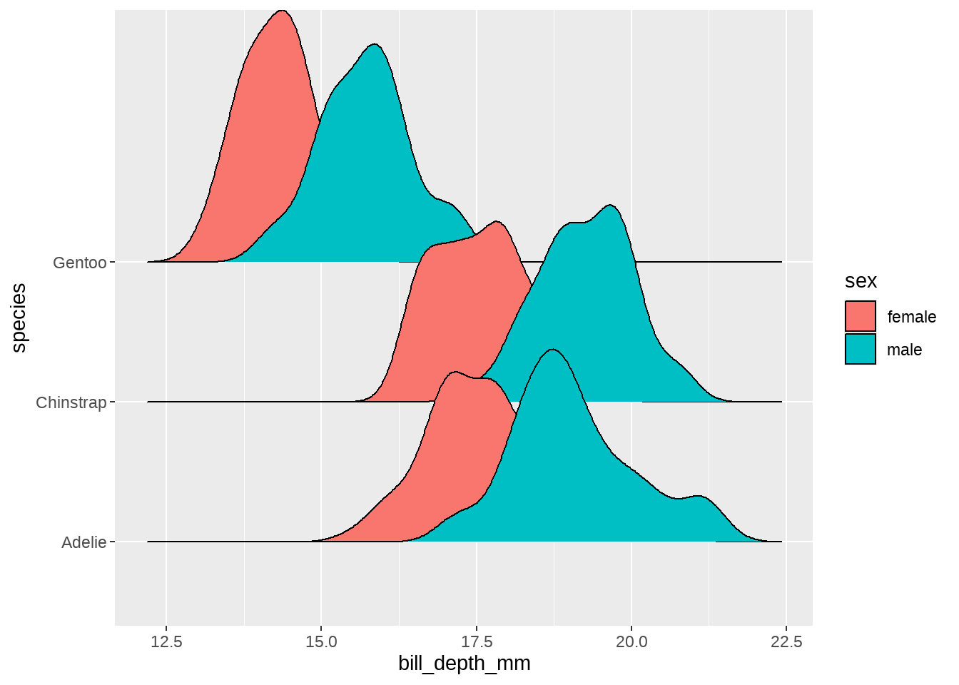

## Picking joint bandwidth of 0.306

penguins %>%
  ggplot(aes(x = body_mass_g, y = species, fill = sex)) +
  ggridges::geom_density_ridges(alpha = 0.5)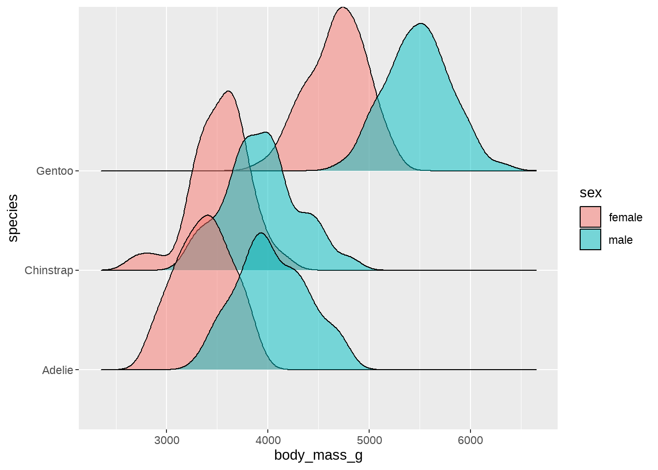

## Picking joint bandwidth of 116

但这样一个特征一个特征的画，好麻烦。你知道程序员都是偷懒的，于是我们还有更骚的操作

penguins %>%
  dplyr::select(species, bill_length_mm:body_mass_g) %>%
  pivot_longer(-species, names_to = "measurement", values_to = "value") %>%
  ggplot(aes(x = value)) +
  geom_density(aes(color = species, fill = species), size = 1.2, alpha = 0.2) +
  facet_wrap(vars(measurement), ncol = 2, scales = "free")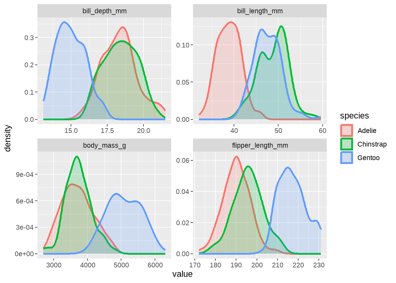

## Warning: Using `size` aesthetic for lines was deprecated in ggplot2 3.4.0.
## ℹ Please use `linewidth` instead.
## This warning is displayed once every 8 hours.
## Call `lifecycle::last_lifecycle_warnings()` to see where this warning was
## generated.

penguins %>%
  dplyr::select(species, bill_length_mm:body_mass_g) %>%
  pivot_longer(-species, names_to = "measurement", values_to = "value") %>%
  ggplot(aes(x = species, y = value)) +
  geom_boxplot(aes(color = species, fill = species), size = 1.2, alpha = 0.2) +
  facet_wrap(vars(measurement), ncol = 2, scales = "free")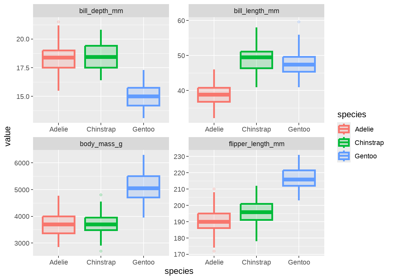

penguins %>%
  dplyr::select(species, bill_length_mm:body_mass_g) %>%
  pivot_longer(-species, names_to = "measurement", values_to = "value") %>%
  ggplot(aes(x = value, y = species, fill = species)) +
  ggridges::geom_density_ridges() +
  facet_wrap(vars(measurement), scales = "free")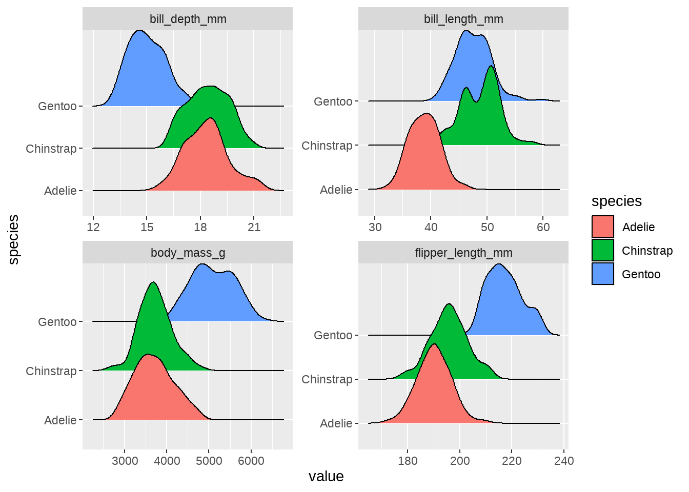

## Picking joint bandwidth of 0.384

## Picking joint bandwidth of 1.08

## Picking joint bandwidth of 153

## Picking joint bandwidth of 2.4

penguins %>%
  dplyr::select(species,sex, bill_length_mm:body_mass_g) %>%
  pivot_longer(
    -c(species, sex), 
    names_to = "measurement", 
    values_to = "value"
    ) %>%
  ggplot(aes(x = value, y = species, fill = sex)) +
  ggridges::geom_density_ridges() +
  facet_wrap(vars(measurement), scales = "free")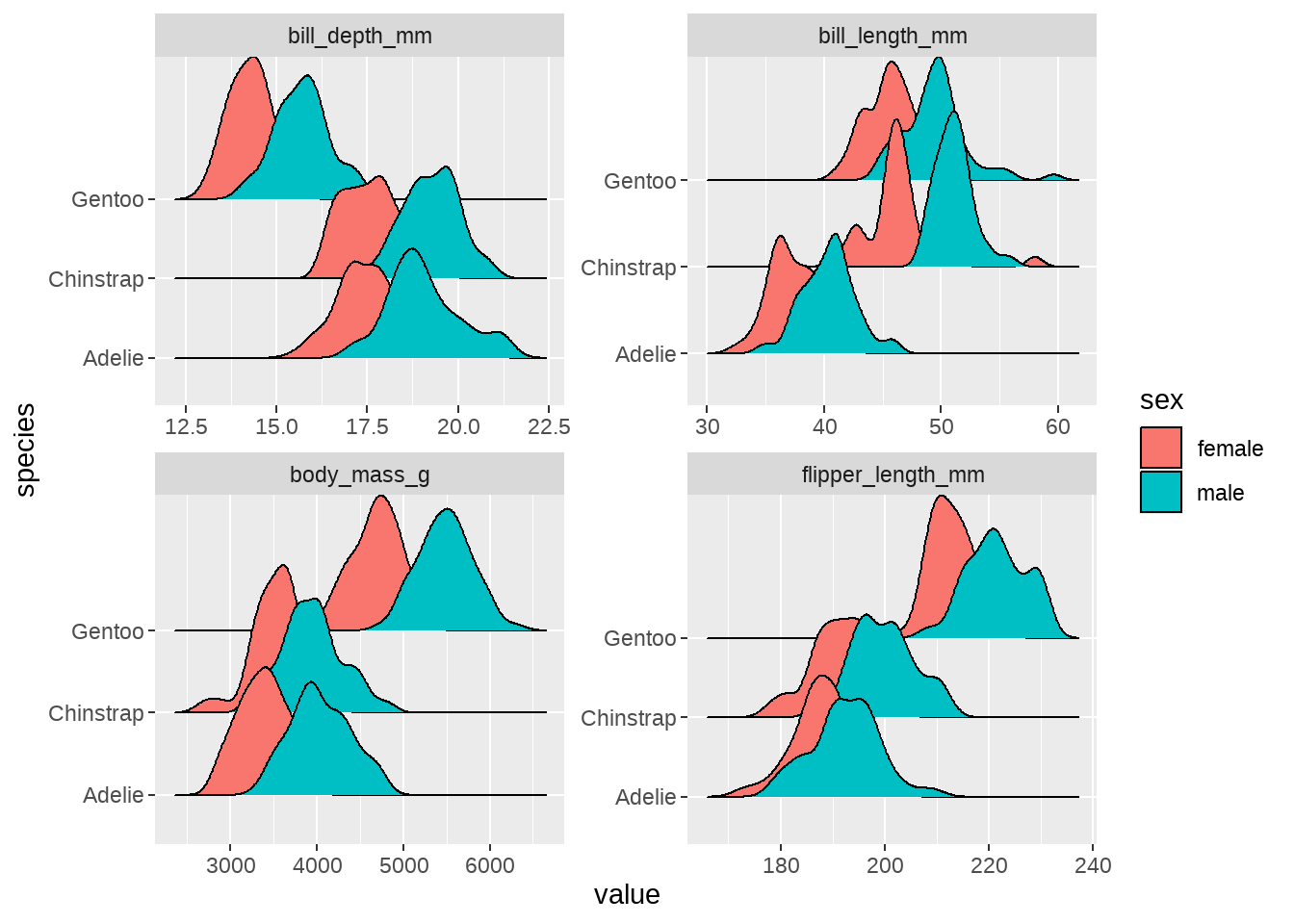

## Picking joint bandwidth of 0.306

## Picking joint bandwidth of 0.717

## Picking joint bandwidth of 116

## Picking joint bandwidth of 2.07

我若有所思的看着这张图，似乎看到了一些特征（pattern）了。

82.2.6 嘴峰长度和深度的关联

嘴巴越长，嘴巴也会越厚？

penguins %>%
  ggplot(aes(
    x = bill_length_mm, y = bill_depth_mm,
    shape = species, color = species
  )) +
  geom_point()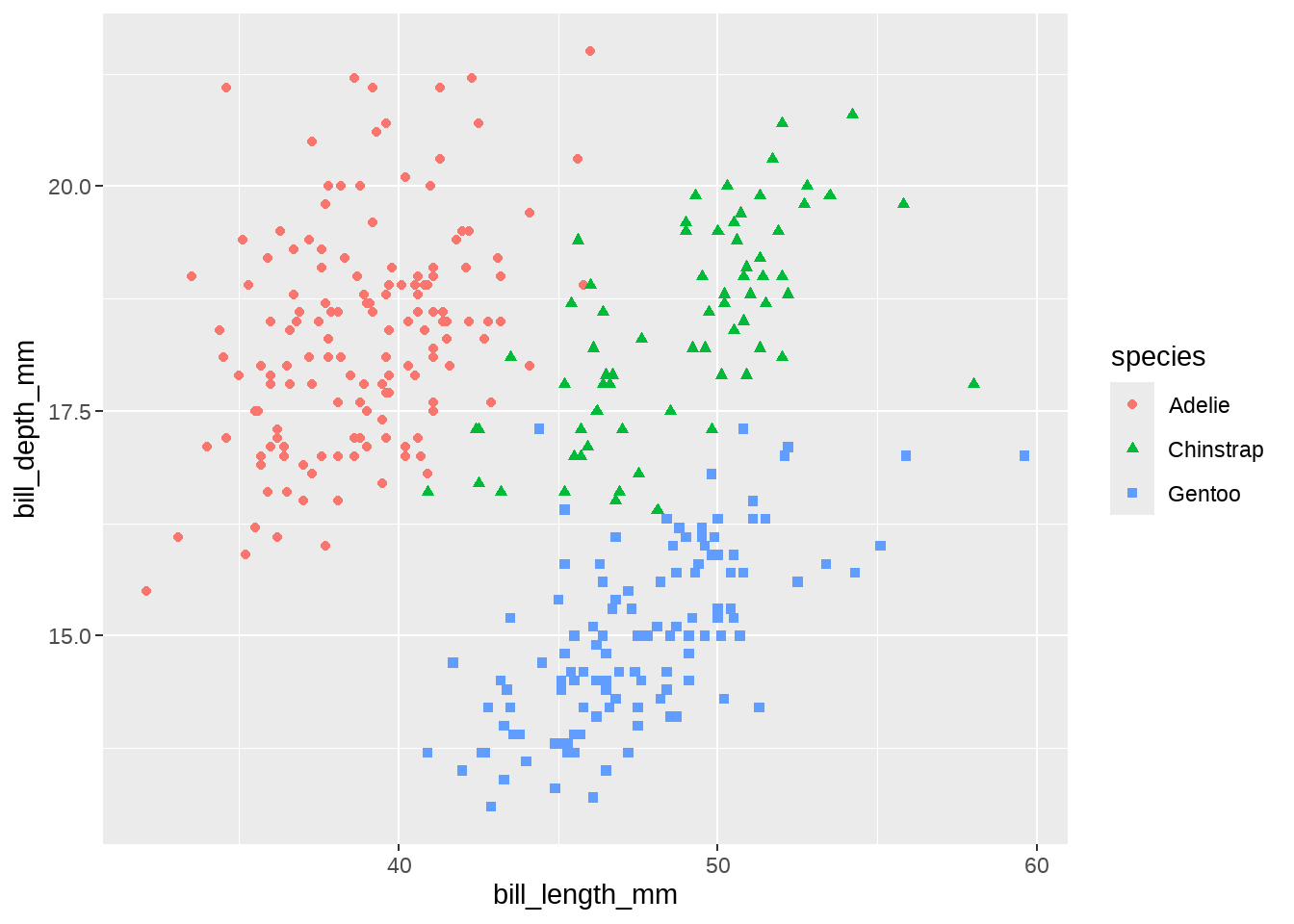

我们把不同的种类，用不同的颜色区分看看

penguins %>%
  ggplot(aes(
    x = bill_length_mm, y = bill_depth_mm,
    shape = species, color = species
  )) +
  geom_point(aes(size = body_mass_g))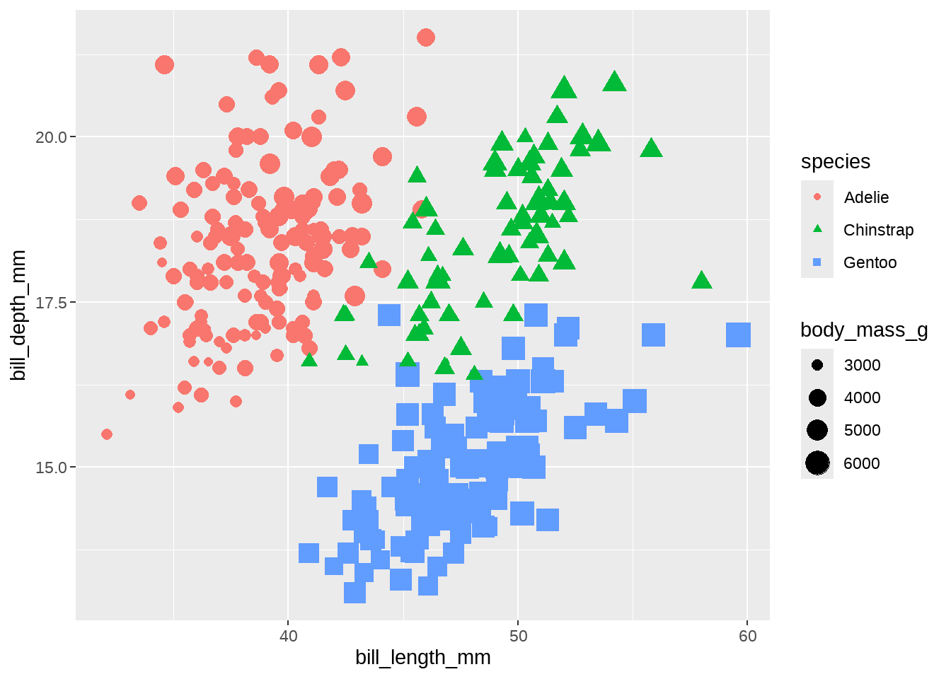

感觉这是一个辛普森佯谬， 我们画图看看

penguins %>%
  ggplot(aes(x = bill_length_mm, y = bill_depth_mm)) +
  geom_point(aes(color = species, shape = species)) +
  geom_smooth(method = lm) +
  geom_smooth(method = lm, aes(color = species))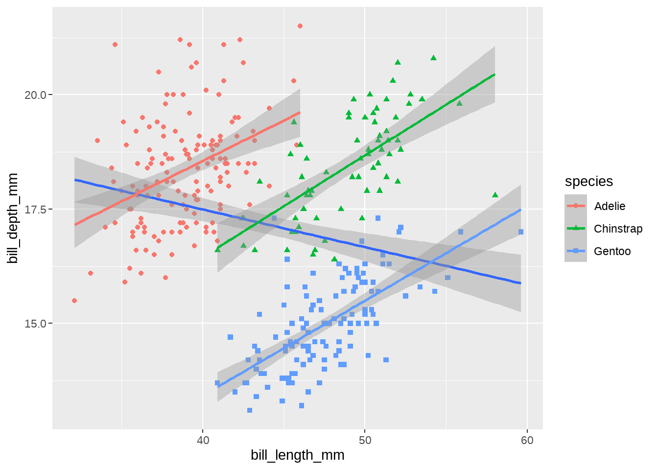

## `geom_smooth()` using formula = 'y ~ x'
## `geom_smooth()` using formula = 'y ~ x'

82.2.7 体重与翅膀长度的关联

翅膀越长，体重越大？

penguins %>%
  group_by(species, island, sex) %>%
  ggplot(aes(
    x = body_mass_g, y = reorder(species, -body_mass_g),
    color = species
  )) +
  geom_jitter(position = position_jitter(seed = 2020, width = 0.2), alpha = 0.4, size = 2) +
  stat_summary(fun = mean, geom = "point", size = 5, alpha = 1)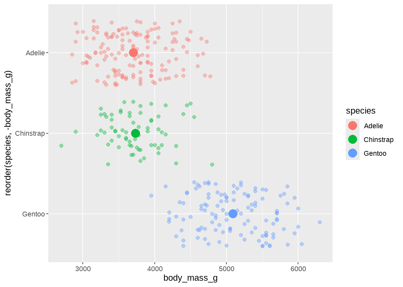

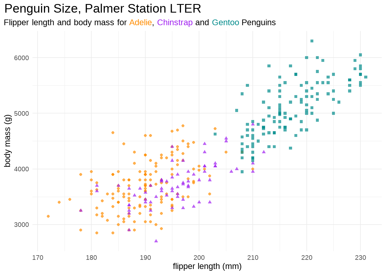
library(ggtext)

## Warning: package 'ggtext' was built under R version 4.2.2

penguins %>%
  ggplot(aes(flipper_length_mm, body_mass_g, group = species)) +
  geom_point(aes(colour = species, shape = species), alpha = 0.7) +
  scale_color_manual(values = c("darkorange", "purple", "cyan4")) +
  labs(
    title = "Penguin Size, Palmer Station LTER",
    subtitle = "Flipper length and body mass for <span style = 'color:darkorange;'>Adelie</span>, <span style = 'color:purple;'>Chinstrap</span> and <span style = 'color:cyan4;'>Gentoo</span> Penguins",
    x = "flipper length (mm)",
    y = "body mass (g)"
  ) +
  theme_minimal() +
  theme(
    legend.position = "none",
    # text = element_text(family = "Futura"),
    # (I only have 'Light' )
    plot.title = element_text(size = 16),
    plot.subtitle = element_markdown(), # element_markdown from `ggtext` to parse the css in the subtitle
    plot.title.position = "plot",
    plot.caption = element_text(size = 8, colour = "grey50"),
    plot.caption.position = "plot"
  )

82.2.8 不同种类的宝宝，体重具有显著性差异？

先分组计算体重的均值和标准差

penguins %>%
  group_by(species) %>%
  summarise(
    count = n(),
    mean_body_mass = mean(body_mass_g),
    sd_body_mass = sd(body_mass_g)
  )

## # A tibble: 3 × 4
##   species   count mean_body_mass sd_body_mass
##   <chr>     <int>          <dbl>        <dbl>
## 1 Adelie      146          3706.         459.
## 2 Chinstrap    68          3733.         384.
## 3 Gentoo      119          5092.         501.

penguins %>%
  ggplot(aes(x = species, y = body_mass_g)) +
  geom_boxplot() +
  geom_jitter()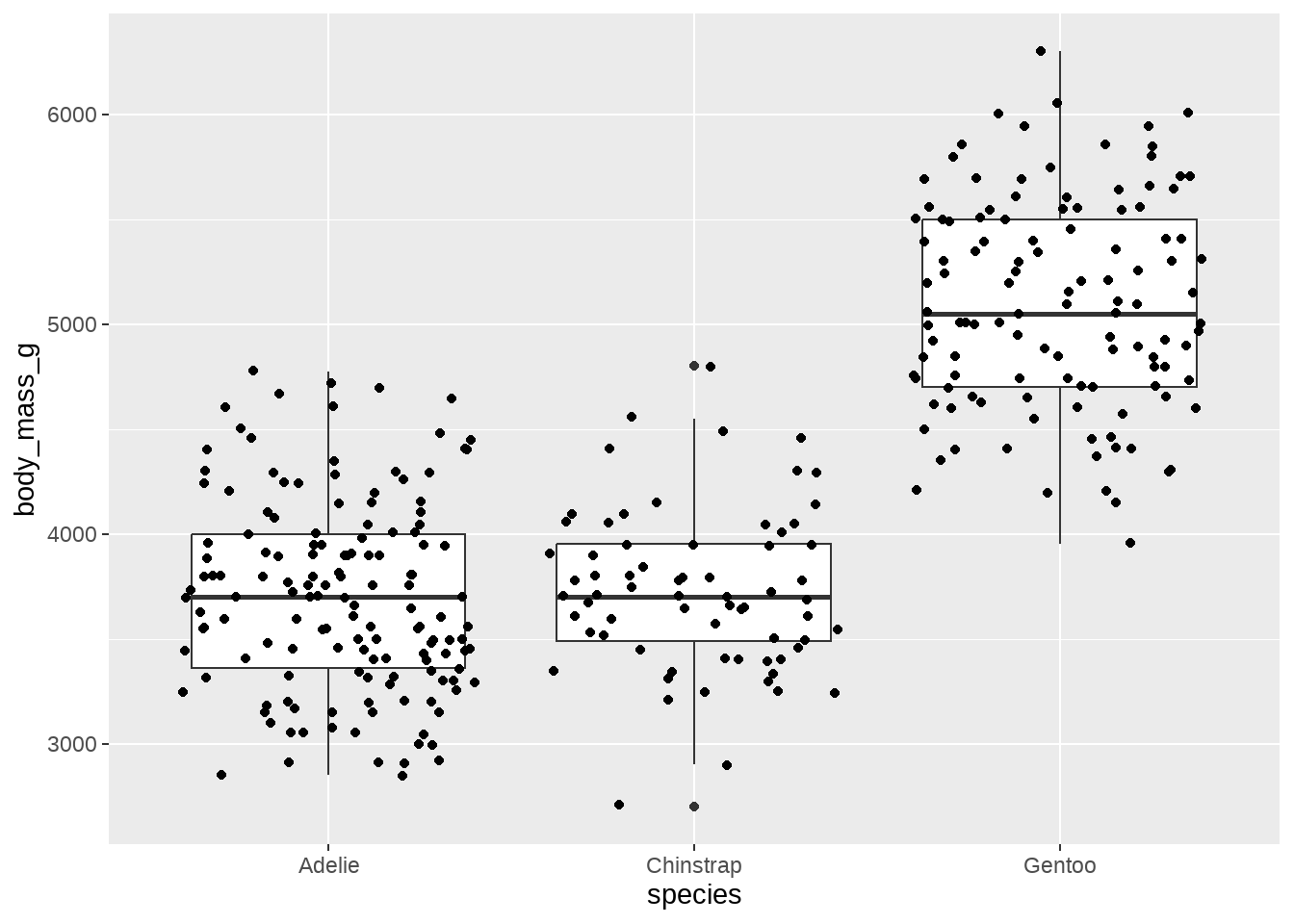

用统计方法验证下我们的猜测吧。记住，我们是有科学精神的的人！

82.2.8.1 参数检验

• one-way ANOVA(要求等方差)

stats::aov(formula = body_mass_g ~ species, data = penguins) %>%
  summary()

##              Df    Sum Sq  Mean Sq F value Pr(>F)    
## species       2 145190219 72595110   341.9 <2e-16 ***
## Residuals   330  70069447   212332                   
## ---
## Signif. codes:  0 '***' 0.001 '**' 0.01 '*' 0.05 '.' 0.1 ' ' 1

p-value 很小，说明不同种类企鹅之间体重是有显著差异的，但aov只给出了species在整体上引起了体重差异（只要有任意两组之间有显著差异，aov给出的p-value都很小），如果想知道不同种类两两之间是否有显著差异，这就需要用到TukeyHSD().

• one-way ANOVA(不要求等方差)，相关介绍看here

oneway.test(body_mass_g ~ species, data = penguins)

## 
##  One-way analysis of means (not assuming equal variances)
## 
## data:  body_mass_g and species
## F = 316.5, num df = 2.00, denom df = 187.68, p-value < 2.2e-16

stats::aov(formula = body_mass_g ~ species, data = penguins) %>%
  TukeyHSD(which = "species") %>%
  broom::tidy()

## # A tibble: 3 × 7
##   term    contrast         null.value estimate conf.low conf.high adj.p.value
##   <chr>   <chr>                 <dbl>    <dbl>    <dbl>     <dbl>       <dbl>
## 1 species Chinstrap-Adelie          0     26.9    -132.      186.    9.16e- 1
## 2 species Gentoo-Adelie             0   1386.     1252.     1520.    5.82e-13
## 3 species Gentoo-Chinstrap          0   1359.     1194.     1524.    5.82e-13

表格第一行instrap-Adelie 的 p-value = 0.916，没通过显著性检验；而Gentoo-Adelie 和 Gentoo-Chinstrap 他们的p-value都接近0，通过显著性检验，这和图中的结果是一致的。

作为统计出生的R语言，有很多宏包可以帮助我们验证我们的结论，我这里推荐可视化学统计的宏包ggstatsplot宏包将统计分析的结果写在图片里，统计结果和图形融合在一起，让统计结果更容易懂了。（使用这个宏包辅助我们学习统计）

library(ggstatsplot)

penguins %>%
  ggstatsplot::ggbetweenstats(
    x = species, # > 2 groups
    y = body_mass_g,
    type = "parametric",
    pairwise.comparisons = TRUE, 
    pairwise.display = "all",
    messages = FALSE,
    var.equal = FALSE
  )

82.2.8.2 非参数检验

相关介绍看here

kruskal.test(body_mass_g ~ species, data = penguins)

## 
##  Kruskal-Wallis rank sum test
## 
## data:  body_mass_g by species
## Kruskal-Wallis chi-squared = 212.09, df = 2, p-value < 2.2e-16

penguins %>%
  ggstatsplot::ggbetweenstats(
    x = species,
    y = body_mass_g,
    type = "nonparametric",
    mean.ci = TRUE,
    pairwise.comparisons = TRUE, # <<
    pairwise.display = "all",    # ns = only non-significant
    p.adjust.method = "fdr",     # <<
    messages = FALSE
  )

哇，原来统计可以这样学！

82.2.9 嘴峰长度与嘴峰深度的比例

penguins %>%
  mutate(ratio = bill_length_mm / bill_depth_mm) %>%
  group_by(species) %>%
  summarise(mean = mean(ratio))

## # A tibble: 3 × 2
##   species    mean
##   <chr>     <dbl>
## 1 Adelie     2.12
## 2 Chinstrap  2.65
## 3 Gentoo     3.18

penguins %>%
  mutate(ratio = bill_length_mm / bill_depth_mm) %>%
  ggplot(aes(x = ratio, fill = species)) +
  ggridges::geom_density_ridges(aes(y = species))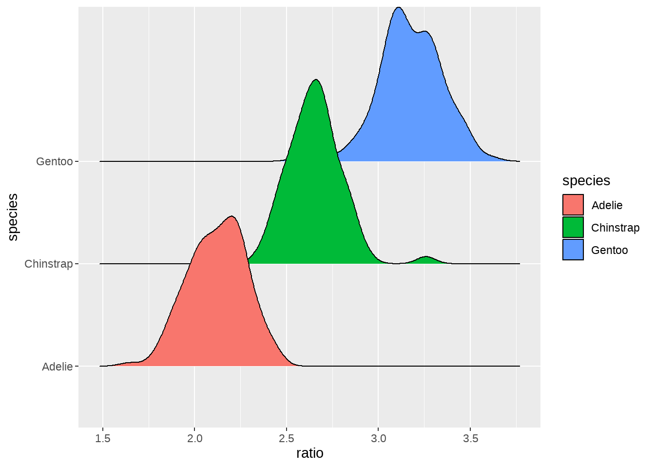

## Picking joint bandwidth of 0.0523

男宝宝和女宝宝颜色区分下，代码只需要修改一个地方，留给大家自己实践下吧。

82.2.10 建立模型

建模需要标准化数据，并对分类变量（比如sex）编码为 1 和 0; （这是第二个好习惯）

scale_fun <- function(x) {  
  (x - mean(x)) / sd(x)
}

d <- penguins %>%
  select(sex, species, bill_length_mm:body_mass_g) %>%
  mutate(
    across(where(is.numeric), scale_fun)
  ) %>%
  mutate(male = if_else(sex == "male", 1, 0))
d

## # A tibble: 333 × 7
##    sex    species bill_length_mm bill_depth_mm flipper_length_mm body_mass_g
##    <chr>  <chr>            <dbl>         <dbl>             <dbl>       <dbl>
##  1 male   Adelie          -0.895         0.780            -1.42       -0.568
##  2 female Adelie          -0.822         0.119            -1.07       -0.506
##  3 female Adelie          -0.675         0.424            -0.426      -1.19 
##  4 female Adelie          -1.33          1.08             -0.568      -0.940
##  5 male   Adelie          -0.858         1.74             -0.782      -0.692
##  6 female Adelie          -0.931         0.323            -1.42       -0.723
##  7 male   Adelie          -0.876         1.24             -0.426       0.581
##  8 female Adelie          -0.529         0.221            -1.35       -1.25 
##  9 male   Adelie          -0.986         2.05             -0.711      -0.506
## 10 male   Adelie          -1.72          2.00             -0.212       0.240
## # ℹ 323 more rows
## # ℹ 1 more variable: male <dbl>

按照species分组后，对flipper_length_mm标准化？这样数据会聚拢到一起了喔, 还是不要了

penguins %>%
  select(sex, species, bill_length_mm:body_mass_g) %>%
  group_by(species) %>%
  mutate(
    across(where(is.numeric), scale_fun)
  ) %>%
  ungroup()

82.2.10.1 model_01

我们将性别sex视为响应变量，其他变量为预测变量。这里性别变量是二元的（0 或者 1），所以我们用logistic回归

logit_mod1 <- glm(
  male ~ 1 + species + bill_length_mm + bill_depth_mm +
    flipper_length_mm + body_mass_g,
  data = d,
  family = binomial(link = "logit")
)

summary(logit_mod1)

## 
## Call:
## glm(formula = male ~ 1 + species + bill_length_mm + bill_depth_mm + 
##     flipper_length_mm + body_mass_g, family = binomial(link = "logit"), 
##     data = d)
## 
## Deviance Residuals: 
##     Min       1Q   Median       3Q      Max  
## -3.3822  -0.2150   0.0023   0.1551   2.8095  
## 
## Coefficients:
##                   Estimate Std. Error z value Pr(>|z|)    
## (Intercept)         4.6835     1.1865   3.947 7.90e-05 ***
## speciesChinstrap   -6.9803     1.5743  -4.434 9.25e-06 ***
## speciesGentoo      -8.3539     2.5235  -3.310 0.000932 ***
## bill_length_mm      3.3566     0.7164   4.685 2.80e-06 ***
## bill_depth_mm       3.1958     0.6546   4.882 1.05e-06 ***
## flipper_length_mm   0.2912     0.6704   0.434 0.664046    
## body_mass_g         4.7228     0.8723   5.414 6.15e-08 ***
## ---
## Signif. codes:  0 '***' 0.001 '**' 0.01 '*' 0.05 '.' 0.1 ' ' 1
## 
## (Dispersion parameter for binomial family taken to be 1)
## 
##     Null deviance: 461.61  on 332  degrees of freedom
## Residual deviance: 127.11  on 326  degrees of freedom
## AIC: 141.11
## 
## Number of Fisher Scoring iterations: 7

计算每个变量的平均边际效应

library(margins)

logit_mod1_m <- logit_mod1 %>% 
 margins() %>% 
 summary() %>% 
 as_tibble()

logit_mod1_m

## # A tibble: 6 × 7
##   factor                AME     SE      z        p   lower   upper
##   <chr>               <dbl>  <dbl>  <dbl>    <dbl>   <dbl>   <dbl>
## 1 bill_depth_mm      0.185  0.0290  6.38  1.82e-10  0.128   0.242 
## 2 bill_length_mm     0.194  0.0339  5.72  1.04e- 8  0.128   0.261 
## 3 body_mass_g        0.273  0.0378  7.22  5.08e-13  0.199   0.347 
## 4 flipper_length_mm  0.0169 0.0388  0.434 6.64e- 1 -0.0592  0.0929
## 5 speciesChinstrap  -0.373  0.0513 -7.27  3.67e-13 -0.473  -0.272 
## 6 speciesGentoo     -0.434  0.0740 -5.86  4.66e- 9 -0.579  -0.289

logit_mod1_m %>%
  ggplot(aes(
    x = reorder(factor, AME),
    y = AME, ymin = lower, ymax = upper
  )) +
  geom_hline(yintercept = 0, color = "gray80") +
  geom_pointrange() +
  coord_flip() +
  labs(x = NULL, y = "Average Marginal Effect")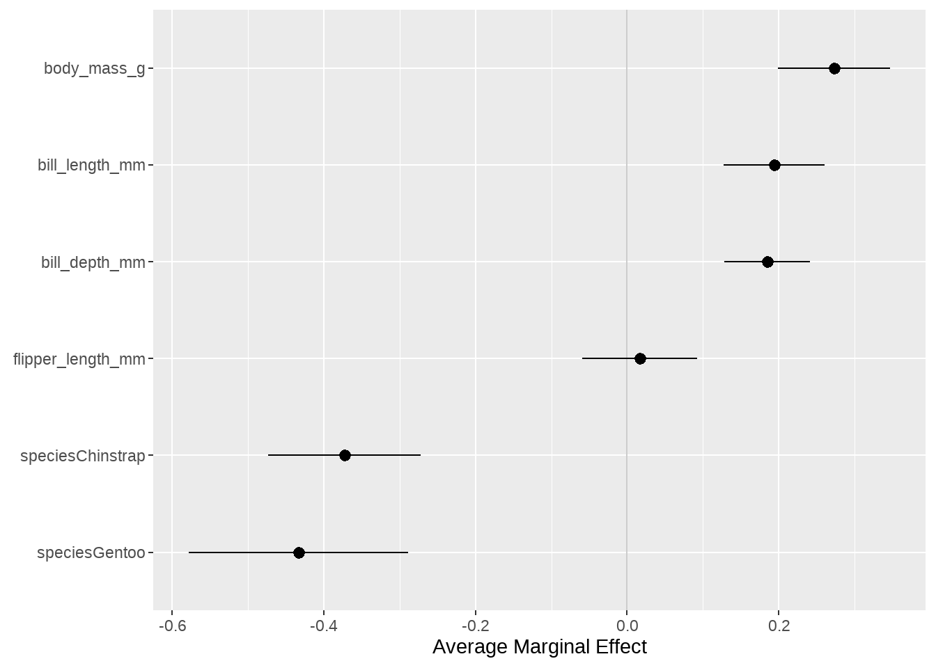

library(ggeffects)
ggpredict(logit_mod1, terms = "bill_length_mm") 

82.2.10.2 model_02

library(brms)

brms_mod2 <- brm(
  male ~ 1 + bill_length_mm + bill_depth_mm + flipper_length_mm + body_mass_g + (1 | species),
  data = d,
  family = binomial(link = "logit")
)

summary(brms_mod2)

library(ggeffects)
ggpredict(brms_mod2, "bill_depth_mm [all]") %>%
  plot()

82.2.10.3 model_03

penguins %>%
  ggplot(aes(x = flipper_length_mm, y = bill_length_mm, color = species)) +
  geom_point()

brms_mod3 <- brm(bill_length_mm ~ flipper_length_mm + (1|species),
  data = penguins
)

penguins %>%
  group_by(species) %>%
  modelr::data_grid(flipper_length_mm) %>%
  tidybayes::add_fitted_draws(brms_mod3, n = 100) %>%
  ggplot() +
  geom_point(
    data = penguins,
    aes(flipper_length_mm, bill_length_mm, color = species, shape = species)
  ) +
  geom_line(aes(flipper_length_mm, .value, group = interaction(.draw, species), color = species), alpha = 0.1)