第 14 章 数据可视化

上节课介绍了R语言的基本数据结构，可能大家有种看美剧的感觉，有些懵。这很正常，我在开始学习R的时候，感觉和大家一样，所以不要惊慌，我们后面会慢慢填补这些知识点。

这节课，我们介绍R语言最强大的可视化，看看都有哪些炫酷的操作。

library(tidyverse) # install.packages("tidyverse")
library(patchwork) # install.packages("patchwork")

14.1 为什么要可视化

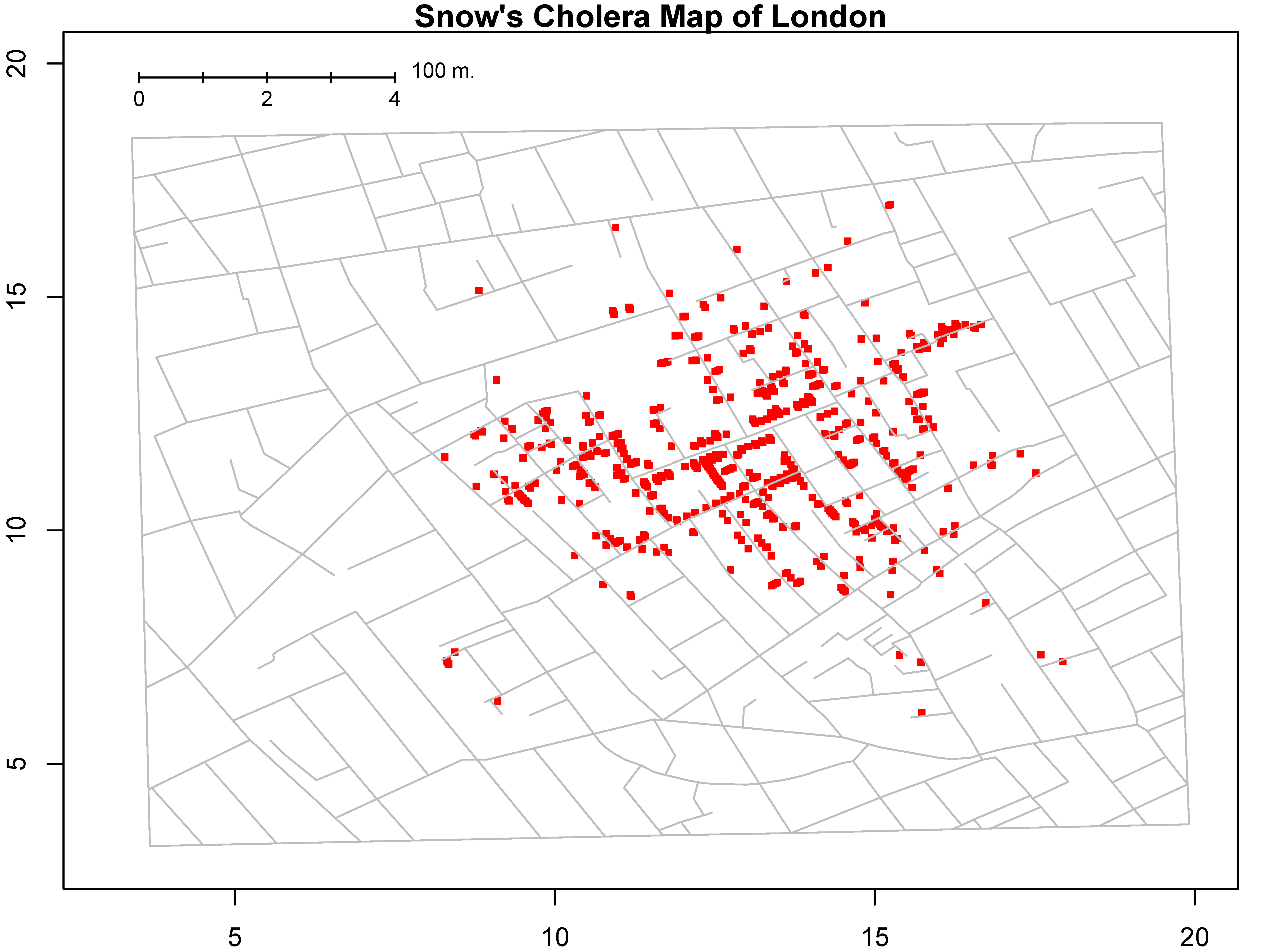
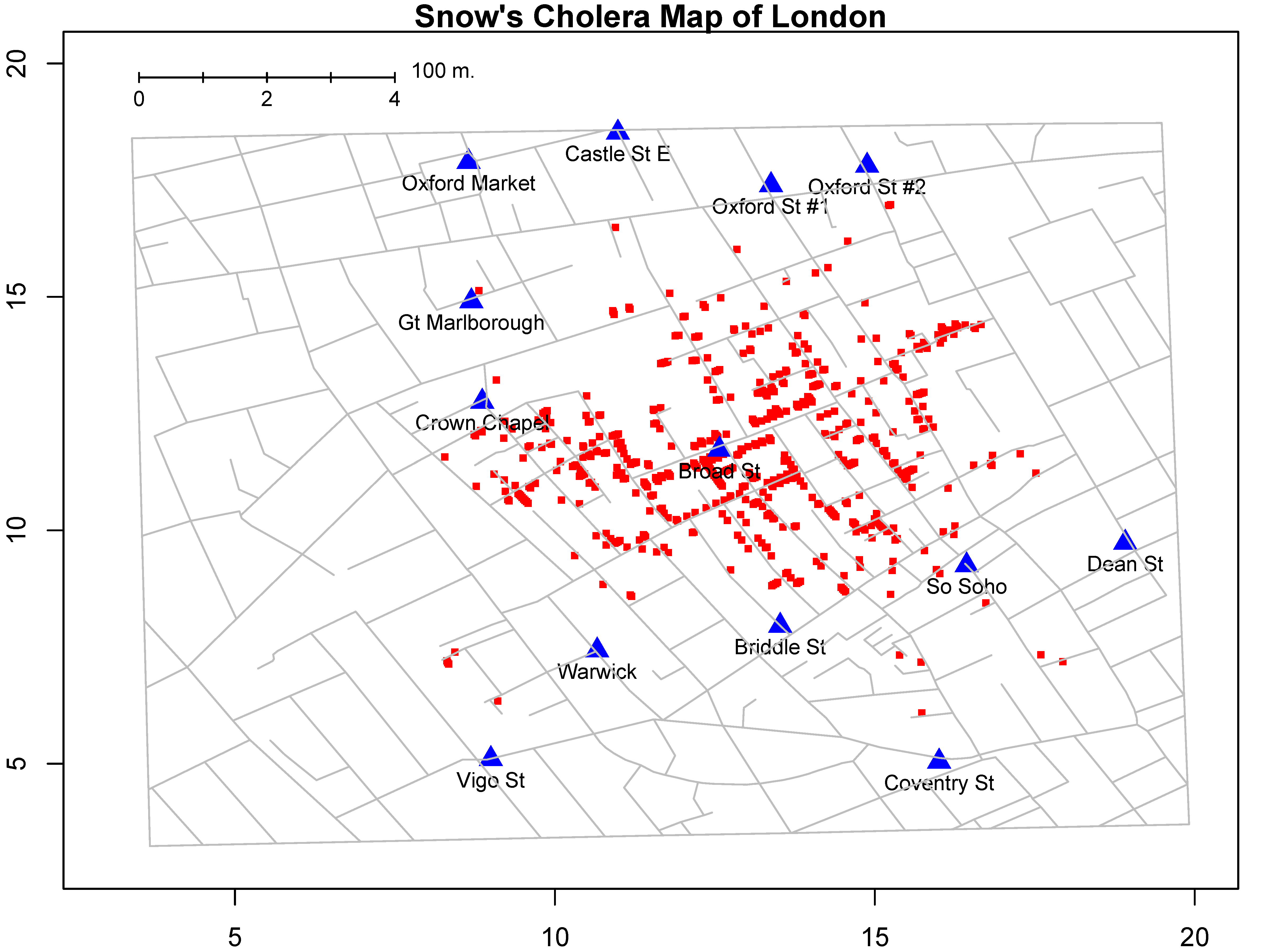
我们先从一个故事开始，1854年伦敦爆发严重霍乱，当时流行的观点是霍乱是通过空气传播的，而John Snow医生（不是《权力的游戏》里的 Jon Snow）研究发现，霍乱是通过饮用水传播的。研究过程中，John Snow医生统计每户病亡人数，每死亡一人标注一条横线，分析发现，大多数病例的住所都围绕在Broad Street水泵附近，结合其他证据得出饮用水传播的结论，于是移掉了Broad Street水泵的把手，霍乱最终得到控制。

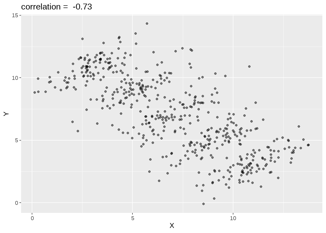
另一个有趣的例子就是辛普森悖论（Simpson’s Paradox）。比如我们想研究下，学习时间和考试成绩的关联。结果发现两者呈负相关性，即补课时间越长，考试成绩反而越差（下图横坐标是学习时间，纵坐标是考试成绩），很明显这个结果有违生活常识。

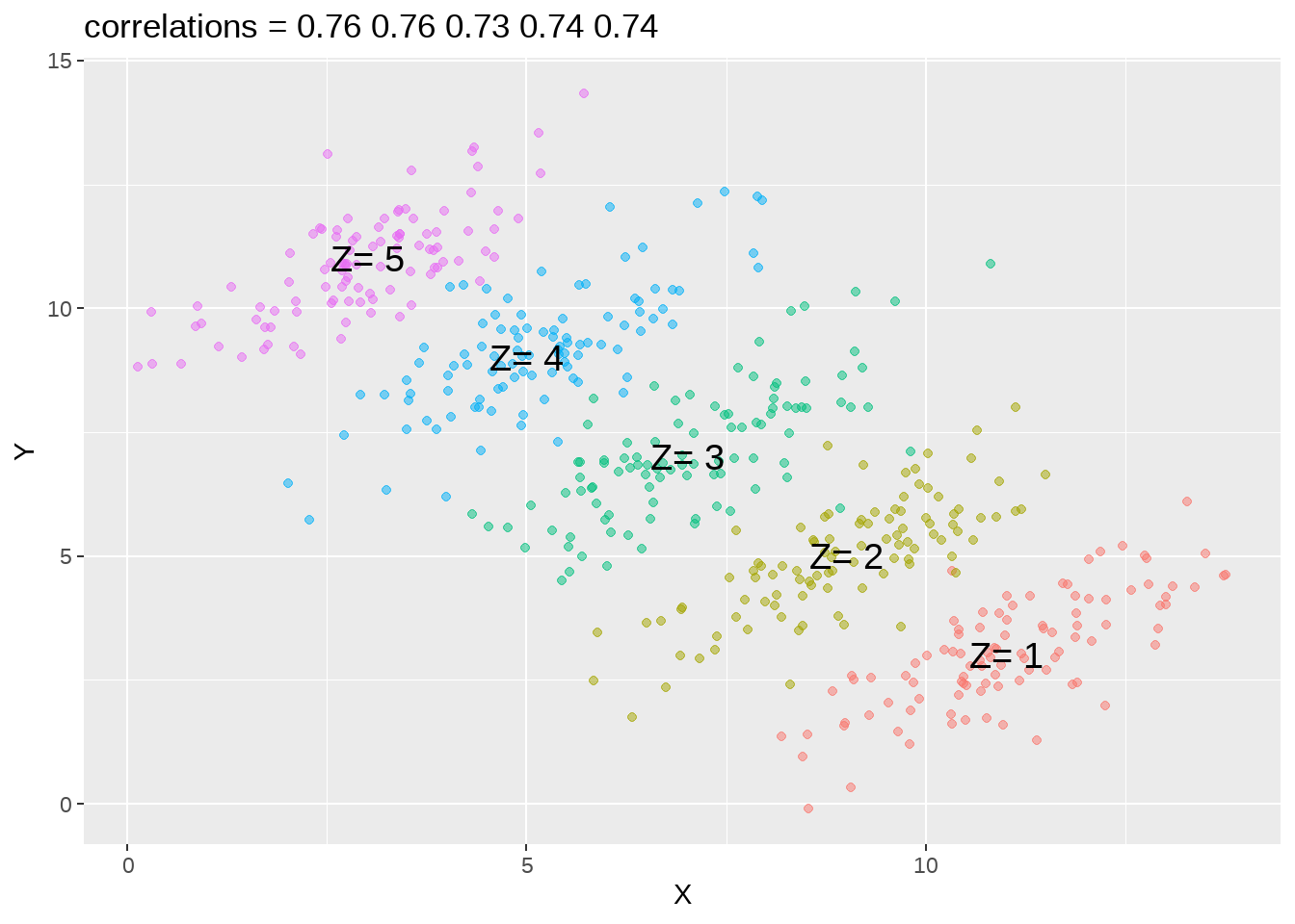
事实上，当我们把学生按照不同年级分成五组，再来观察学习时间和考试成绩之间的关联，发现相关性完全逆转了! 我们可以看到学习时间和考试成绩强烈正相关。

辛普森悖论在日常生活中层出不穷。 那么如何避免辛普森悖论呢？我们能做的，就是仔细地研究分析各种影响因素，不要笼统概括地、浅尝辄止地看问题。其中，可视化分析为我们提供了一个好的方法。

14.2 什么是数据可视化

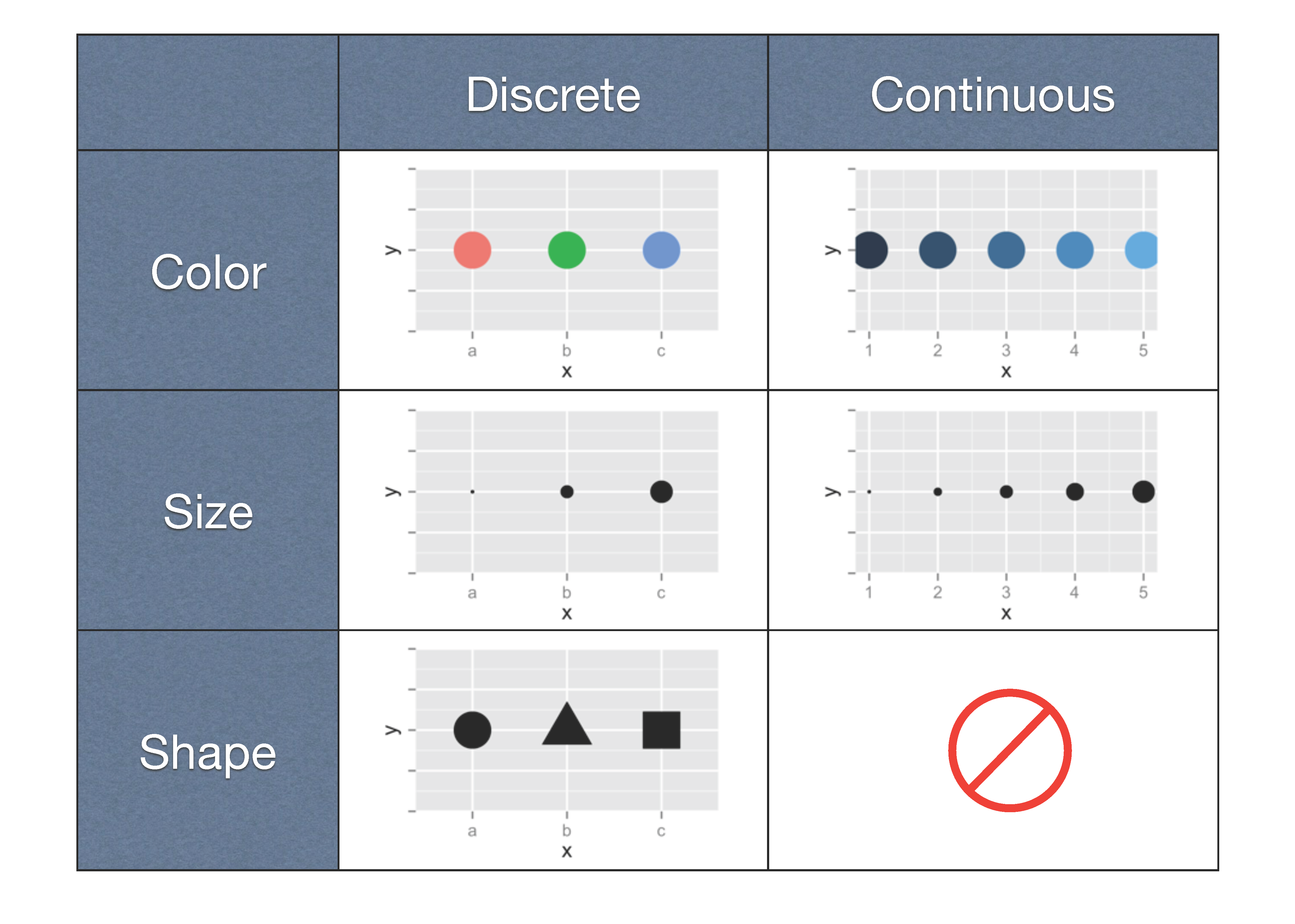
14.2.1 图形属性(视觉元素)

我们在图中画一个点，那么这个点就有（形状，大小，颜色，位置，透明度）等属性， 这些属性就是图形属性（有时也称之为图形元素或者视觉元素），下图 14.1列出了常用的图形属性。

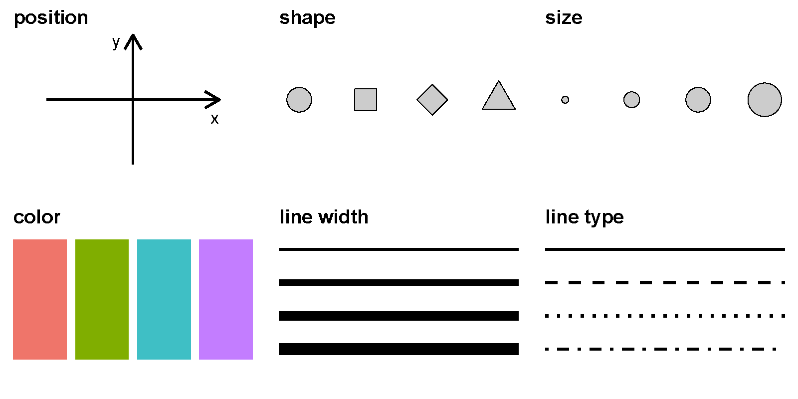
图 14.1: 常用的图形元素

点和线常用的图形属性

geom	x	y	size	color	shape	linetype	alpha	fill	group
point	√	√	√	√	√	√	√	√	√
line	√	√	√	√		√	√		√

14.3 宏包ggplot2

ggplot2是RStudio首席科学家Hadley Wickham在2005年读博士期间的作品。很多人学习R语言，就是因为ggplot2宏包。目前， ggplot2已经发展成为最受欢迎的R宏包，没有之一。我们可以看看它2019年cran的下载量

library(cranlogs)

d <- cran_downloads(package = "ggplot2", from = "2019-01-01", to = "2019-12-31")

sum(d$count)

## [1] 9889742

14.3.1 ggplot2 的图形语法

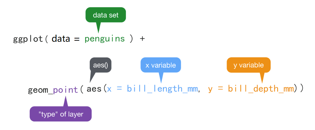
ggplot2有一套优雅的绘图语法，包名中“gg”是grammar of graphics的简称。 Hadley Wickham将这套可视化语法诠释为:

一张统计图形就是从数据到几何形状(geometric object，缩写geom)所包含的图形属性(aesthetic attribute，缩写aes)的一种映射。

通俗解释：就是我们的数据通过图形的视觉元素表示出来。比如点的位置，如果坐标x值越大，水平方向离原点的位置就越远，数值越小，水平方向离原点的位置就越近。 数值的大小变成了视觉能感知的东西。

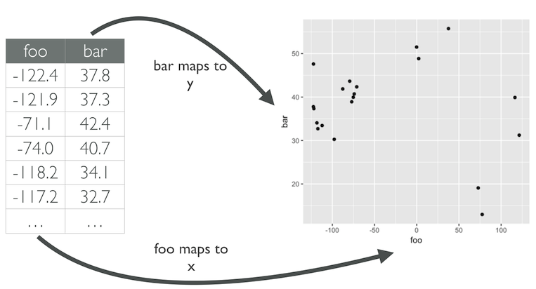
图 14.2: 数值到图形属性的映射过程

同理，我们希望用点的大小代表这个位置上的某个变量（比如，降雨量，产品销量等等），那么变量的数值越小，点的半径就小一点，数值越大，点就可以大一点；或者变量的数值大，点的颜色就深一点，数值小，点的颜色就浅一点。即，数值到图形属性的映射过程。映射是一个数学词汇，这里您可以理解为一一对应。

14.3.2 怎么写代码

ggplot()函数包括9个部件：

• 数据 (data) （数据框）
• 映射 (mapping)
• 几何形状 (geom)
• 统计变换 (stats)
• 标度 (scale)
• 坐标系 (coord)
• 分面 (facet)
• 主题 (theme)
• 存储和输出 (output)

其中前三个是必需的。语法模板

ggplot(data = <DATA>) + 
   <GEOM_FUNCTION>(mapping = aes(<MAPPINGS>))

此外，图形中还可能包含数据的统计变换(statistical transformation，缩写stats)，最后绘制在某个特定的坐标系(coordinate system，缩写coord)中，而分面(facet)则可以用来生成数据不同子集的图形。

先来点小菜。先看一个简单的案例（1880-2014年温度变化和二氧化碳排放量）

library(tidyverse)
d <- read_csv(here::here("demo_data", "temp_carbon.csv"))
d %>% head(5)

## # A tibble: 5 × 5
##    year temp_anomaly land_anomaly ocean_anomaly carbon_emissions
##   <dbl>        <dbl>        <dbl>         <dbl>            <dbl>
## 1  1880        -0.11        -0.48         -0.01              236
## 2  1881        -0.08        -0.4           0.01              243
## 3  1882        -0.1         -0.48          0                 256
## 4  1883        -0.18        -0.66         -0.04              272
## 5  1884        -0.26        -0.69         -0.14              275

library(ggplot2)
ggplot(___) + 
  geom_point(
    mapping = aes(x = ___, y = ___)
  )

我们只需要在相应位置填入数据框，和数据框的变量，就可以画图

ggplot(data = d) +
  geom_point(mapping = aes(x = year, y = carbon_emissions)) +
  xlab("Year") +
  ylab("Carbon emissions (metric tons)") +
  ggtitle("Annual global carbon emissions, 1880-2014")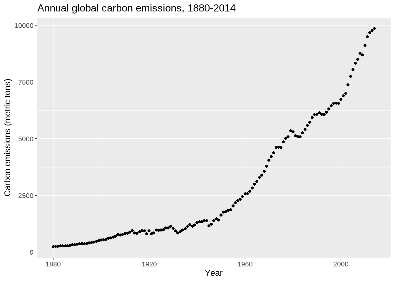

是不是很简单?

14.4 映射

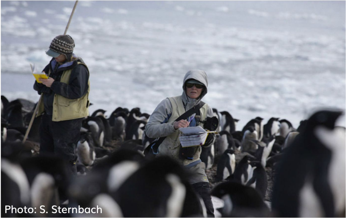
我们这里用科考人员收集的企鹅体征数据来演示。

library(tidyverse)
penguins <- read_csv(here::here("demo_data", "penguins.csv")) %>%
  janitor::clean_names() %>% 
  drop_na()

penguins %>%
  head()

## # A tibble: 6 × 8
##   species island    bill_length_mm bill_depth_mm flipper_length_mm body_mass_g
##   <chr>   <chr>              <dbl>         <dbl>             <dbl>       <dbl>
## 1 Adelie  Torgersen           39.1          18.7               181        3750
## 2 Adelie  Torgersen           39.5          17.4               186        3800
## 3 Adelie  Torgersen           40.3          18                 195        3250
## 4 Adelie  Torgersen           36.7          19.3               193        3450
## 5 Adelie  Torgersen           39.3          20.6               190        3650
## 6 Adelie  Torgersen           38.9          17.8               181        3625
## # ℹ 2 more variables: sex <chr>, year <dbl>

14.4.1 变量含义

variable	class	description
species	character	企鹅种类 (Adelie, Gentoo, Chinstrap)
island	character	所在岛屿 (Biscoe, Dream, Torgersen)
bill_length_mm	double	嘴峰长度 (单位毫米)
bill_depth_mm	double	嘴峰深度 (单位毫米)
flipper_length_mm	integer	鰭肢长度 (单位毫米)
body_mass_g	integer	体重 (单位克)
sex	character	性别
year	integer	记录年份

我们会用到penguins数据集其中的四个变量

penguins %>%
  select(species, sex, bill_length_mm, bill_depth_mm) %>%
  head(4)

14.4.2 嘴巴越长，嘴巴也会越厚？

这里提出一个问题，嘴巴越长，嘴巴也会越厚？

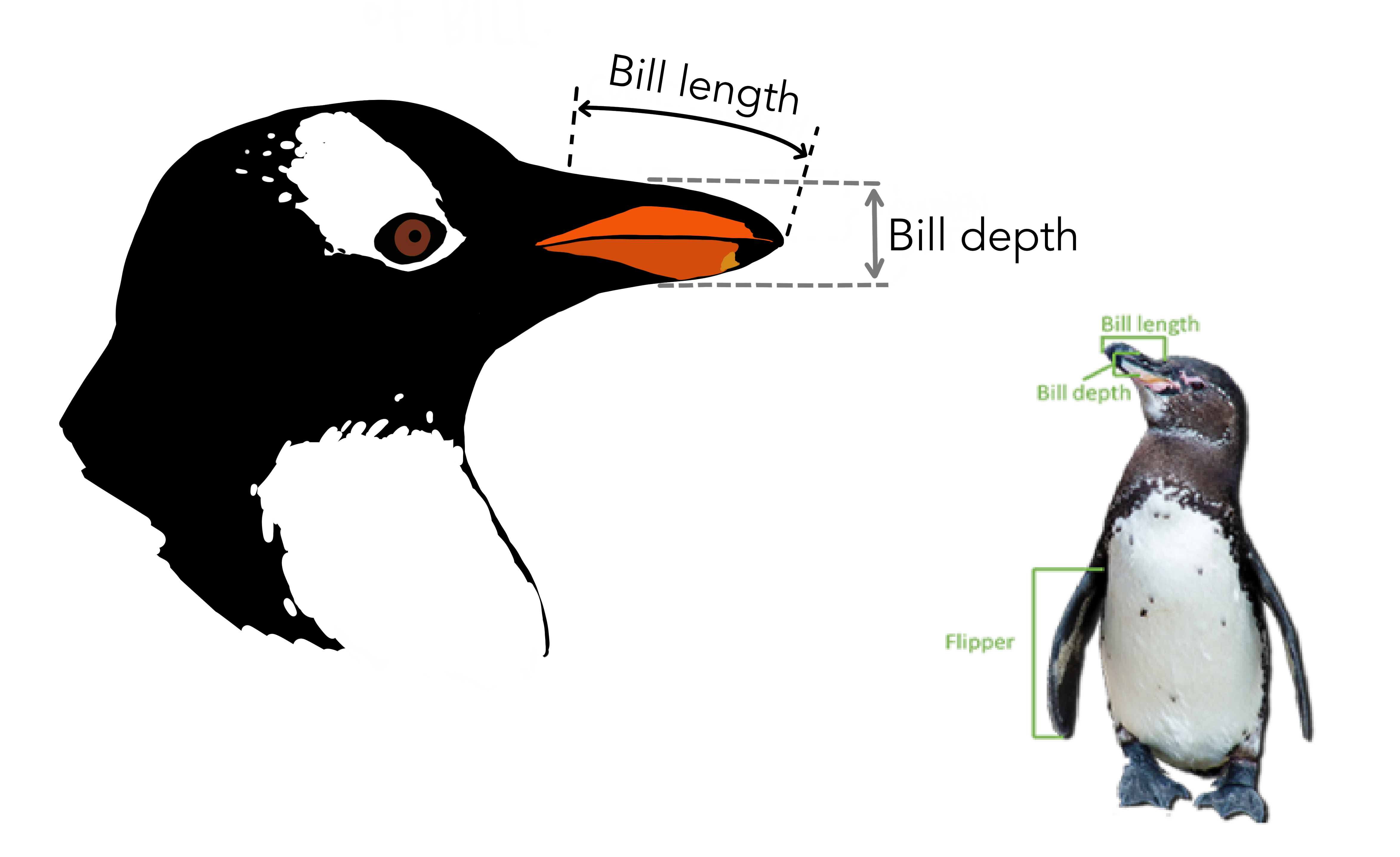
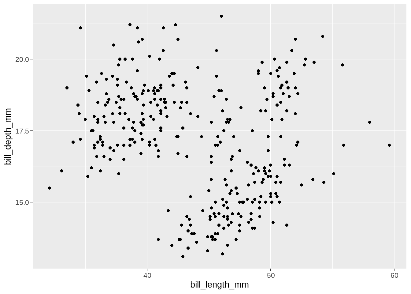
为考察嘴峰长度(bill_length_mm)与嘴峰深度(bill_depth_mm)之间的关联，先绘制这两个变量的散点图，

• ggplot() 初始化绘图，相当于打开了一张纸，准备画画。

• ggplot(data = penguins) 表示使用penguins这个数据框来画图。

• +表示添加图层。

• geom_point()表示绘制散点图。

• aes()表示数值和视觉属性之间的映射。

aes(x = bill_length_mm, y = bill_depth_mm)，意思是变量bill_length_mm作为（映射为）x轴方向的位置，变量bill_depth_mm作为（映射为）y轴方向的位置。

• aes()除了位置上映射，还可以实现色彩、形状或透明度等视觉属性的映射。

运行脚本后生成图片：

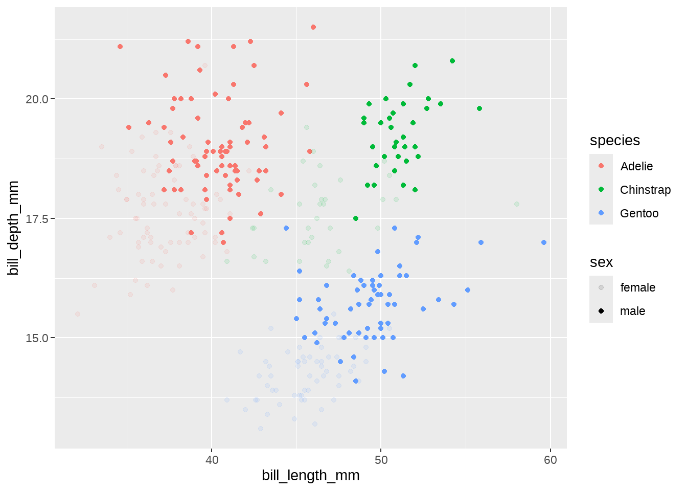
刚才看到的是位置上的映射，ggplot()还包含了颜色、形状以及透明度等图形属性的映射，

比如我们在aes()里增加一个颜色映射color = species, 这样做就是希望，不同的企鹅类型, 用不同的颜色来表现。这里，企鹅类型有三组，那么就用三种不同的颜色来表示

ggplot(penguins) +
  geom_point(aes(x = bill_length_mm, y = bill_depth_mm, color = species))

此图绘制不同类型的企鹅，嘴峰长度与嘴峰深度散点图，并用颜色来实现了分组。

大家试试下面代码呢，

ggplot(penguins) +
  geom_point(aes(x = bill_length_mm, y = bill_depth_mm, size = species))

ggplot(penguins) +
  geom_point(aes(x = bill_length_mm, y = bill_depth_mm, shape = species))

ggplot(penguins) +
  geom_point(aes(x = bill_length_mm, y = bill_depth_mm, alpha = species))

也可更多映射

ggplot(penguins) +
  geom_point(
    aes(x = bill_length_mm, y = bill_depth_mm, color = species, alpha = sex)
  )

## Warning: Using alpha for a discrete variable is not advised.

为什么图中是这样的颜色呢？那是因为ggplot()内部有一套默认的设置

不喜欢默认的颜色，可以自己定义喔。请往下看

14.5 映射 vs.设置

想把图中的点指定为某一种颜色，可以使用设置语句，比如

ggplot(penguins) +
  geom_point(aes(x = bill_length_mm, y = bill_depth_mm), color = "blue")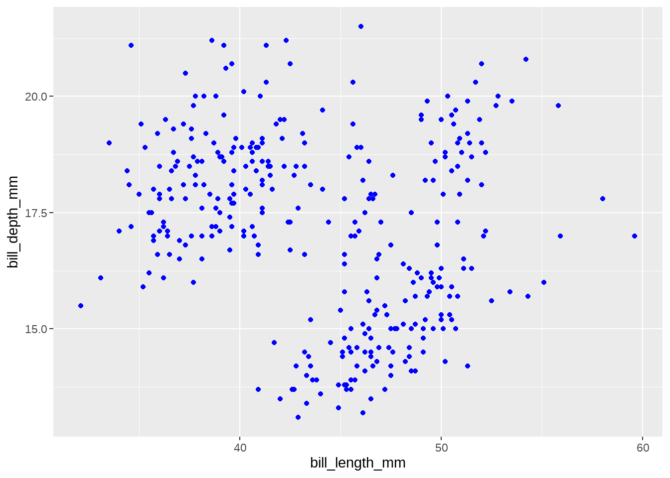

大家也可以试试下面

ggplot(penguins) +
  geom_point(aes(x = bill_length_mm, y = bill_depth_mm), size = 5)

ggplot(penguins) +
  geom_point(aes(x = bill_length_mm, y = bill_depth_mm), shape = 2)

ggplot(penguins) +
  geom_point(aes(x = bill_length_mm, y = bill_depth_mm), alpha = 0.5)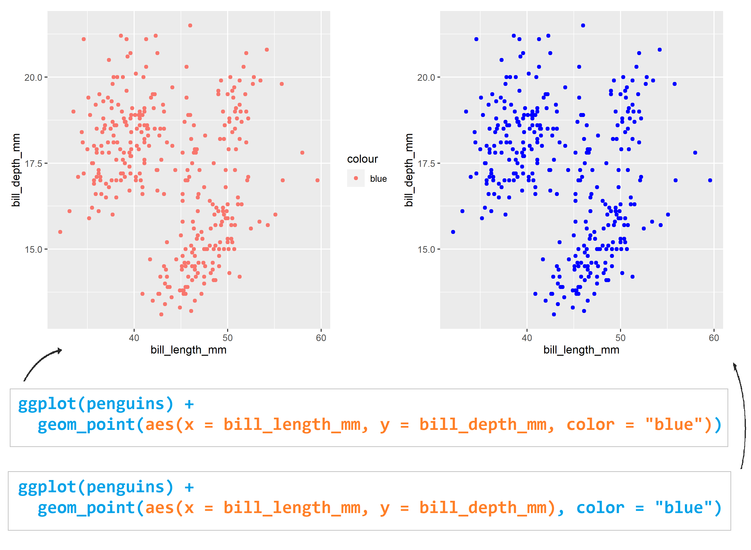

14.5.1 提问

思考下左图中aes(color = "blue")为什么会变成了红色的点？

14.6 几何形状

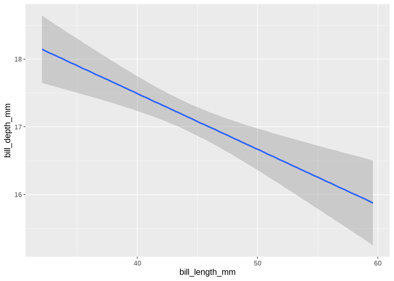
geom_point() 可以画散点图，也可以使用geom_smooth()绘制平滑曲线，

ggplot(penguins) +
  geom_smooth(aes(x = bill_length_mm, y = bill_depth_mm))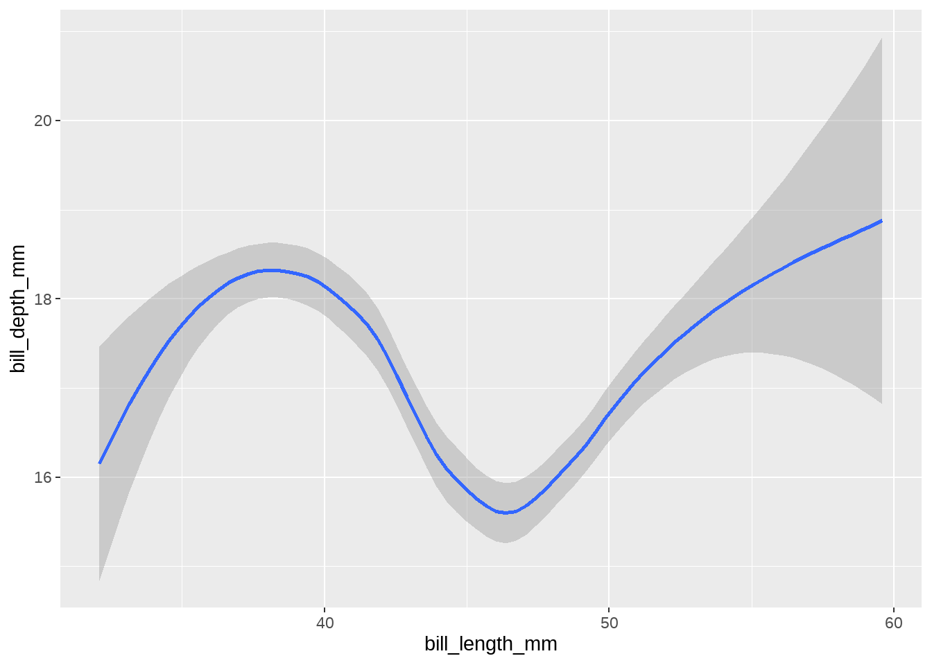

## `geom_smooth()` using method = 'loess' and formula = 'y ~ x'

ggplot(penguins) +
  geom_smooth(
    aes(x = bill_length_mm, y = bill_depth_mm),
    method = "lm"
   )

## `geom_smooth()` using formula = 'y ~ x'

14.7 图层叠加

ggplot(penguins) +
  geom_point(aes(x = bill_length_mm, y = bill_depth_mm)) +
  geom_smooth(aes(x = bill_length_mm, y = bill_depth_mm))

## `geom_smooth()` using method = 'loess' and formula = 'y ~ x'

很强大，但相同的代码让我写两遍，我不高兴。要在偷懒的路上追求简约

ggplot(penguins, aes(x = bill_length_mm, y = bill_depth_mm)) +
  geom_point() +
  geom_smooth()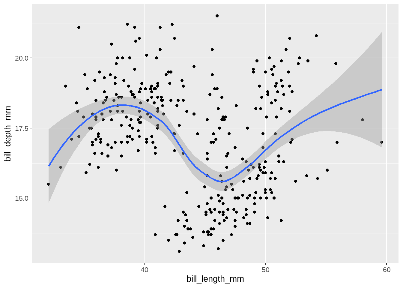

## `geom_smooth()` using method = 'loess' and formula = 'y ~ x'

以上两段代码出来的图为什么是一样？背后的含义有什么不同？接着往下看

14.8 Global vs. Local

ggplot(penguins, aes(x = bill_length_mm, y = bill_depth_mm, color = species)) +
  geom_point()

ggplot(penguins) +
  geom_point(aes(x = bill_length_mm, y = bill_depth_mm, color = species))

大家可以看到，以上两段代码出来的图是一样。但背后的含义却不同。

• 映射关系aes(x = bill_length_mm, y = bill_depth_mm) 写在ggplot()里, 为全局声明。那么，当geom_point()画图时，发现缺少图形所需要的映射关系（点的位置、点的大小、点的颜色等等），就会从ggplot()全局变量中继承映射关系。

• 如果映射关系aes(x = bill_length_mm, y = bill_depth_mm) 写在几何形状geom_point()里, 那么此处的映射关系就为局部声明, 那么geom_point()绘图时，发现所需要的映射关系已经存在，就不会继承全局变量的映射关系。

看下面这个例子，

ggplot(penguins, aes(x = bill_length_mm, y = bill_depth_mm)) +
  geom_point(aes(color = species)) +
  geom_smooth()

这里的 geom_point() 和 geom_smooth() 都会从全局变量中继承位置映射关系。

再看下面这个例子，

ggplot(penguins,aes(x = bill_length_mm, y = bill_depth_mm, color = species)) +
  geom_point(aes(color = sex))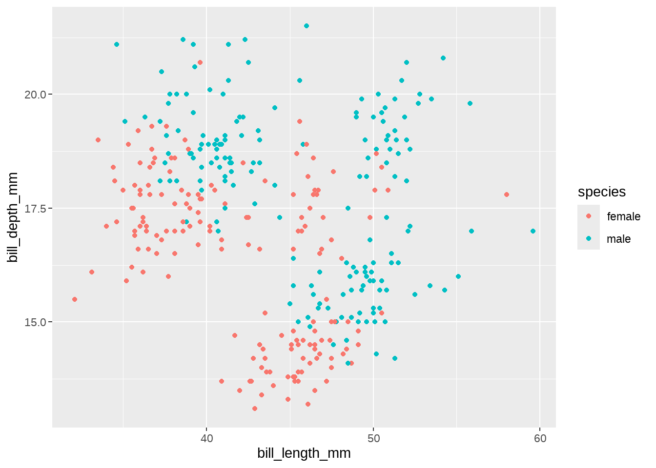

局部变量中的映射关系 aes(color = )已经存在，因此不会从全局变量中继承，沿用当前的映射关系。

14.8.1 图层从全局声明中继承

体会下代码之间的区别

ggplot(penguins, aes(x = bill_length_mm, y = bill_depth_mm, color = species)) +
  geom_point()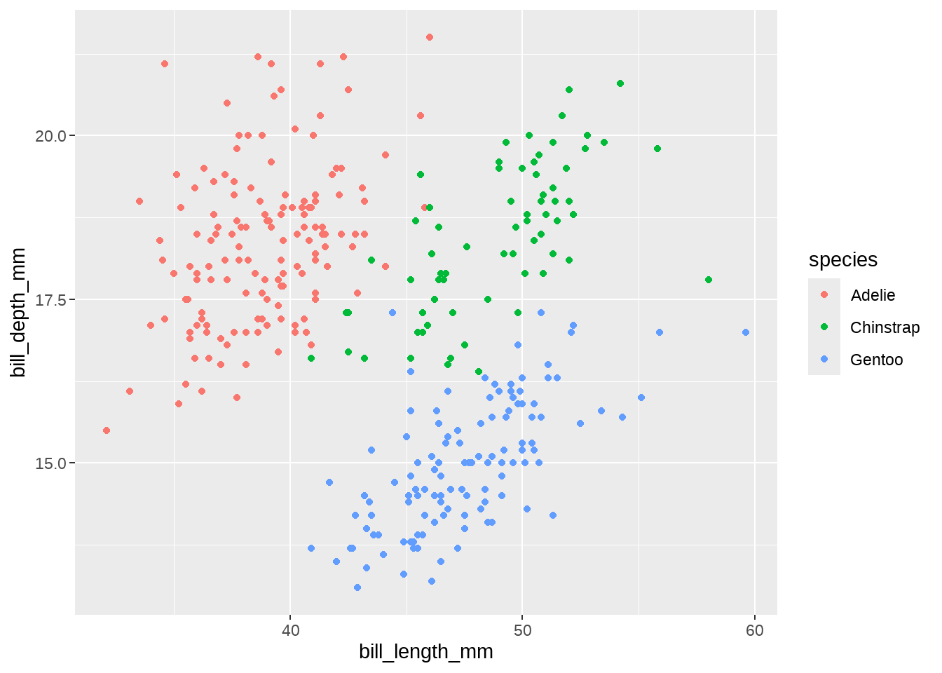

ggplot(penguins, aes(x = bill_length_mm, y = bill_depth_mm)) +
  geom_point(aes(color = species))

ggplot(penguins, aes(x = bill_length_mm, y = bill_depth_mm, color = sex)) +
  geom_point(aes(color = species))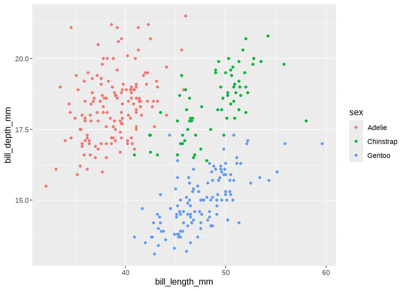

14.8.2 图层之间没有继承关系

再看下面这个例子

ggplot(penguins, aes(x = bill_length_mm, y = bill_depth_mm)) +
  geom_point() +
  geom_smooth(method = "lm")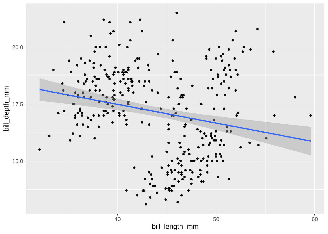

## `geom_smooth()` using formula = 'y ~ x'

ggplot(penguins, aes(x = bill_length_mm, y = bill_depth_mm)) +
  geom_point(aes(color = species)) +
  geom_smooth(method = "lm")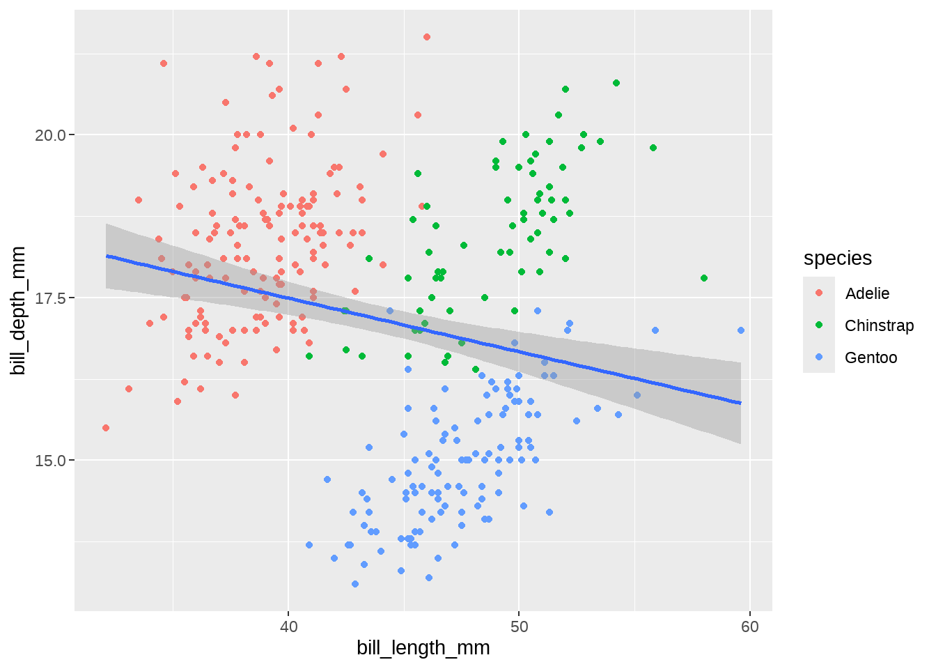

## `geom_smooth()` using formula = 'y ~ x'

ggplot(penguins, aes(x = bill_length_mm, y = bill_depth_mm)) +
  geom_smooth(method = "lm") +
  geom_point(aes(color = species))

## `geom_smooth()` using formula = 'y ~ x'

ggplot(penguins, aes(x = bill_length_mm, y = bill_depth_mm, color = species)) +
  geom_point() +
  geom_smooth(method = "lm")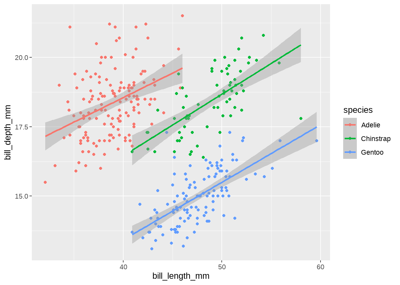 

## `geom_smooth()` using formula = 'y ~ x'

ggplot(penguins, aes(x = bill_length_mm, y = bill_depth_mm, color = species)) +
  geom_point(aes(color = sex)) +
  geom_smooth(method = "lm")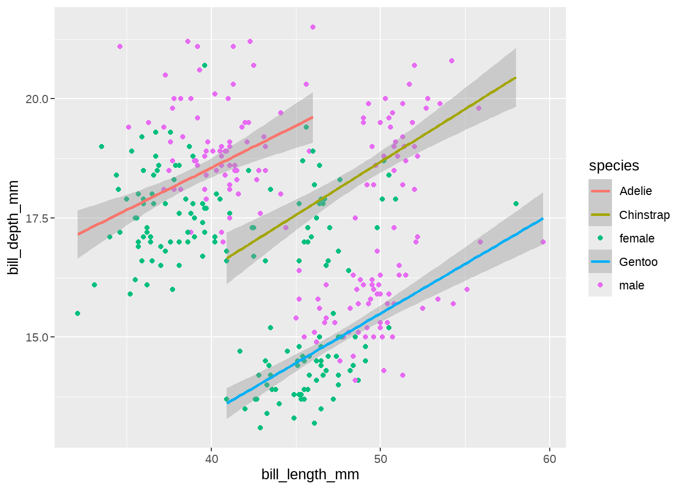 

## `geom_smooth()` using formula = 'y ~ x'

ggplot(penguins, aes(x = bill_length_mm, y = bill_depth_mm, color = species)) +
  geom_point() +
  geom_smooth(method = "lm", aes(color = sex))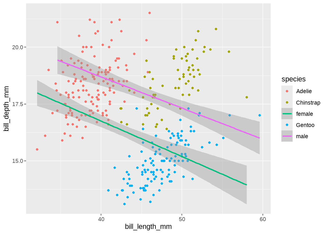 

## `geom_smooth()` using formula = 'y ~ x'

14.9 保存图片

可以使用ggsave()函数，将图片保存为所需要的格式，如”.pdf”, “.png”等， 还可以指定图片的高度和宽度，默认units是英寸，也可以使用”cm”, or “mm”.

p1 <- penguins %>% 
  ggplot(aes(x = bill_length_mm, y = bill_depth_mm)) +
  geom_smooth(method = lm) +
  geom_point(aes(color = species)) +
  ggtitle("This is my first plot")

ggsave(
  plot = p1,
  filename = "my_plot.pdf",
  width = 8,
  height = 6,
  dpi = 300
)

如果想保存当前图形，ggplot() 也可以不用赋值，同时省略ggsave()中的 plot = p1，ggsave()会自动保存最近一次的绘图

penguins %>% 
  ggplot(aes(x = bill_length_mm, y = bill_depth_mm)) +
  geom_smooth(method = lm) +
  geom_point(aes(color = species)) +
  ggtitle("This is my first plot")

ggsave("my_last_plot.pdf", width = 8, height = 6, dpi = 300)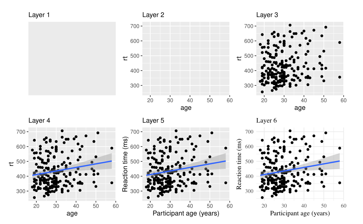

14.10 课堂作业

补充代码，要求在一张图中画出

• 企鹅嘴巴长度和嘴巴厚度的散点图
• 不同企鹅种类用不同的颜色
• 整体的线性拟合
• 不同种类分别线性拟合

ggplot(penguins, aes(x = ___, y = ___)) +
  geom_point() +
  geom_smooth() +
  geom_smooth() 

14.11 小结

图 14.3: Evolution of a layered plot

14.12 延伸阅读

在第 22 章到第 26 章会再讲ggplot2

• 一个点有位置、颜色、大小、形状外，还有哪些属性？如果画线条，应该有哪些视觉属性？
  • 打开 https://ggplot2tor.com/aesthetics
  • 输入 geom_point 或者 geom_line 试试
• https://osf.io/bj83f/
• https://ggplot2.tidyverse.org/

## Warning in rm(corrs, d, dat, data, means, penguins, N, p, p1, p2, p3, Sigma):
## object 'p1' not found

## Warning in rm(corrs, d, dat, data, means, penguins, N, p, p1, p2, p3, Sigma):
## object 'p2' not found

## Warning in rm(corrs, d, dat, data, means, penguins, N, p, p1, p2, p3, Sigma):
## object 'p3' not found