第 79 章 探索性数据分析-奥林匹克
这是Nature期刊上的一篇文章Nature. 2004 September 30; 431(7008),
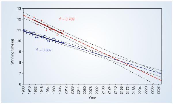
虽然觉得这个结论不太严谨,但我却无力反驳。
于是在文章补充材料里,我找到了文章使用的数据,现在的任务是,重复这张图和文章的分析过程。
79.1 导入数据
d <- read_excel("./demo_data/olympics.xlsx")
d
## # A tibble: 27 × 3
## Olympic_year Men_score Women_score
## <dbl> <dbl> <dbl>
## 1 1900 11 NA
## 2 1904 11 NA
## 3 1908 10.8 NA
## 4 1912 10.8 NA
## 5 1916 NA NA
## 6 1920 10.8 NA
## 7 1924 10.6 NA
## 8 1928 10.8 12.2
## 9 1932 10.3 11.9
## 10 1936 10.3 11.5
## # ℹ 17 more rows79.2 可视化
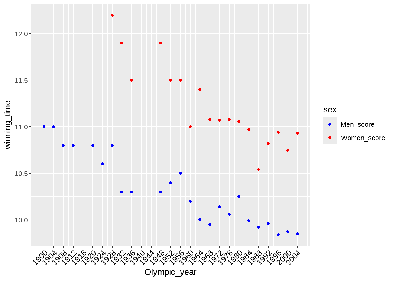
我们先画图看看
d %>%
ggplot() +
geom_point(aes(x = Olympic_year, y = Men_score), color = "blue") +
geom_point(aes(x = Olympic_year, y = Women_score), color = "red")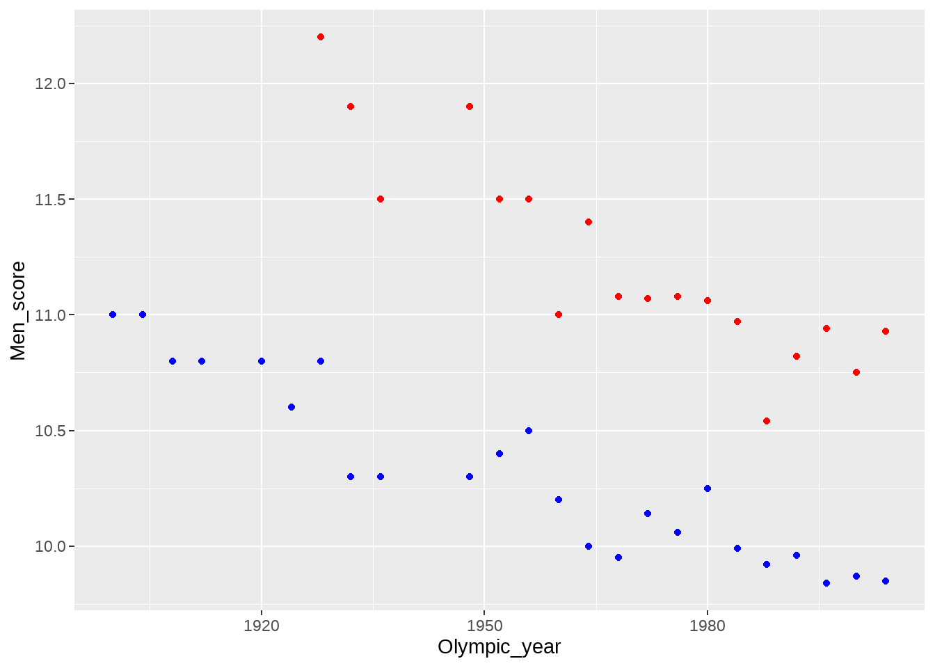 这样写也是可以的,只不过最好先tidy数据
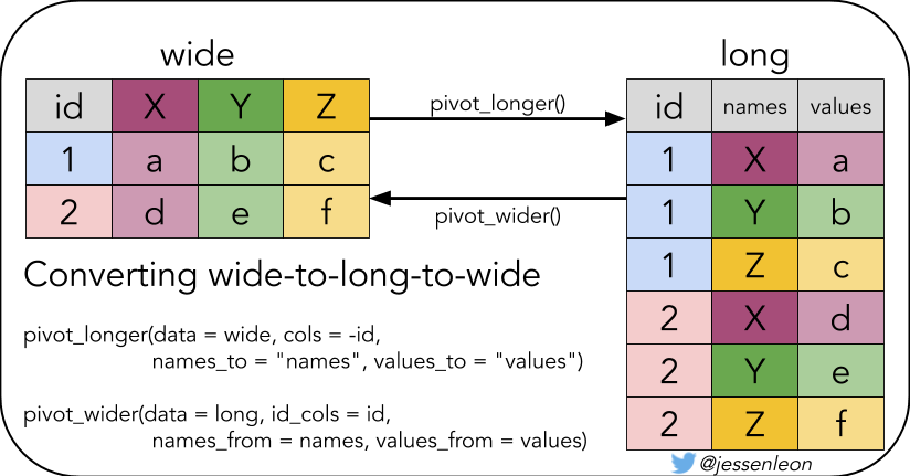
d1 <- d %>%
  pivot_longer(
    cols = -Olympic_year,
    names_to = "sex",
    values_to = "winning_time"
  )

d1
## # A tibble: 54 × 3
## Olympic_year sex winning_time
## <dbl> <chr> <dbl>
## 1 1900 Men_score 11
## 2 1900 Women_score NA
## 3 1904 Men_score 11
## 4 1904 Women_score NA
## 5 1908 Men_score 10.8
## 6 1908 Women_score NA
## 7 1912 Men_score 10.8
## 8 1912 Women_score NA
## 9 1916 Men_score NA
## 10 1916 Women_score NA
## # ℹ 44 more rows然后在画图
d1 %>%
  ggplot(aes(x = Olympic_year, y = winning_time, color = sex)) +
  geom_point() +
  # geom_smooth(method = "lm") +
  scale_color_manual(
    values = c("Men_score" = "blue", "Women_score" = "red")
  ) +
  scale_x_continuous(
    breaks = seq(1900, 2004, by = 4),
    labels = seq(1900, 2004, by = 4)
  ) +
  theme(axis.text.x = element_text(
    size = 10, angle = 45, colour = "black",
    vjust = 1, hjust = 1
  ))
79.3 回归分析
建立年份与成绩的线性关系 \[ \text{score}_i = \alpha + \beta \times \text{year}_i + \epsilon_i; \qquad \epsilon_i\in \text{Normal}(\mu, \sigma) \]
我们需要求出其中系数\(\alpha\)和\(\beta\),写R语言代码如下
(lm(y ~ 1 + x,data = d), 要求得 \(\alpha\)和\(\beta\),就是对应 1 和 x 前的系数)
##
## Call:
## lm(formula = Men_score ~ 1 + Olympic_year, data = d)
##
## Residuals:
##       Min        1Q    Median        3Q       Max
## -0.263708 -0.052702  0.007381  0.080048  0.214559
##
## Coefficients:
##                Estimate Std. Error t value Pr(>|t|)
## (Intercept)  31.8264525  1.6796428   18.95 4.11e-15 ***
## Olympic_year -0.0110056  0.0008593  -12.81 1.13e-11 ***
## ---
## Signif. codes:  0 '***' 0.001 '**' 0.01 '*' 0.05 '.' 0.1 ' ' 1
##
## Residual standard error: 0.1347 on 22 degrees of freedom
##   (3 observations deleted due to missingness)
## Multiple R-squared:  0.8817, Adjusted R-squared:  0.8764
## F-statistic: 164 on 1 and 22 DF, p-value: 1.128e-11##
## Call:
## lm(formula = Women_score ~ 1 + Olympic_year, data = d)
##
## Residuals:
## Min 1Q Median 3Q Max
## -0.37579 -0.08460 0.00929 0.08285 0.32234
##
## Coefficients:
## Estimate Std. Error t value Pr(>|t|)
## (Intercept) 44.347049 4.284251 10.35 1.70e-08 ***
## Olympic_year -0.016822 0.002176 -7.73 8.63e-07 ***
## ---
## Signif. codes: 0 '***' 0.001 '**' 0.01 '*' 0.05 '.' 0.1 ' ' 1
##
## Residual standard error: 0.2104 on 16 degrees of freedom
## (9 observations deleted due to missingness)
## Multiple R-squared: 0.7888, Adjusted R-squared: 0.7756
## F-statistic: 59.76 on 1 and 16 DF, p-value: 8.626e-0779.4 预测
使用predict()完成预测
df <- data.frame(Olympic_year = 2020)

predict(fit_1, newdata = df)
## 1
## 9.595218为了图片中的一致,我们使用1900年到2252年(seq(1900, 2252, by = 4))建立预测项,并整理到数据框里
grid <- tibble(
  Olympic_year = as.numeric(seq(1900, 2252, by = 4))
)
grid
## # A tibble: 89 × 1
## Olympic_year
## <dbl>
## 1 1900
## 2 1904
## 3 1908
## 4 1912
## 5 1916
## 6 1920
## 7 1924
## 8 1928
## 9 1932
## 10 1936
## # ℹ 79 more rows
tb <- grid %>%
  mutate(
    Predict_Men = predict(fit_1, newdata = grid),
    Predict_Women = predict(fit_2, newdata = grid)
  )
tb
## # A tibble: 89 × 3
## Olympic_year Predict_Men Predict_Women
## <dbl> <dbl> <dbl>
## 1 1900 10.9 12.4
## 2 1904 10.9 12.3
## 3 1908 10.8 12.3
## 4 1912 10.8 12.2
## 5 1916 10.7 12.1
## 6 1920 10.7 12.0
## 7 1924 10.7 12.0
## 8 1928 10.6 11.9
## 9 1932 10.6 11.8
## 10 1936 10.5 11.8
## # ℹ 79 more rows有时候我喜欢用modelr::add_predictions()函数实现相同的功能
library(modelr)
grid %>%
  add_predictions(fit_1, var = "Predict_Men") %>%
  add_predictions(fit_2, var = "Predict_Women")
## # A tibble: 89 × 3
## Olympic_year Predict_Men Predict_Women
## <dbl> <dbl> <dbl>
## 1 1900 10.9 12.4
## 2 1904 10.9 12.3
## 3 1908 10.8 12.3
## 4 1912 10.8 12.2
## 5 1916 10.7 12.1
## 6 1920 10.7 12.0
## 7 1924 10.7 12.0
## 8 1928 10.6 11.9
## 9 1932 10.6 11.8
## 10 1936 10.5 11.8
## # ℹ 79 more rows79.5 再次可视化
tb1 <- tb %>%
  pivot_longer(
    cols = -Olympic_year,
    names_to = "sex",
    values_to = "winning_time"
  )
tb1
## # A tibble: 178 × 3
## Olympic_year sex winning_time
## <dbl> <chr> <dbl>
## 1 1900 Predict_Men 10.9
## 2 1900 Predict_Women 12.4
## 3 1904 Predict_Men 10.9
## 4 1904 Predict_Women 12.3
## 5 1908 Predict_Men 10.8
## 6 1908 Predict_Women 12.3
## 7 1912 Predict_Men 10.8
## 8 1912 Predict_Women 12.2
## 9 1916 Predict_Men 10.7
## 10 1916 Predict_Women 12.1
## # ℹ 168 more rows
tb1 %>%
ggplot(aes(
x = Olympic_year,
y = winning_time,
color = sex
)) +
geom_line(size = 2) +
geom_point(data = d1) +
scale_color_manual(
values = c(
"Men_score" = "blue",
"Women_score" = "red",
"Predict_Men" = "#588B8B",
"Predict_Women" = "#C8553D"
),
labels = c(
"Men_score" = "Men score",
"Women_score" = "Women score",
"Predict_Men" = "Men Predict score",
"Predict_Women" = "Women Predict score"
)
) +
scale_x_continuous(
breaks = seq(1900, 2252, by = 16),
labels = as.character(seq(1900, 2252, by = 16))
) +
theme(axis.text.x = element_text(
size = 10, angle = 45, colour = "black",
vjust = 1, hjust = 1
))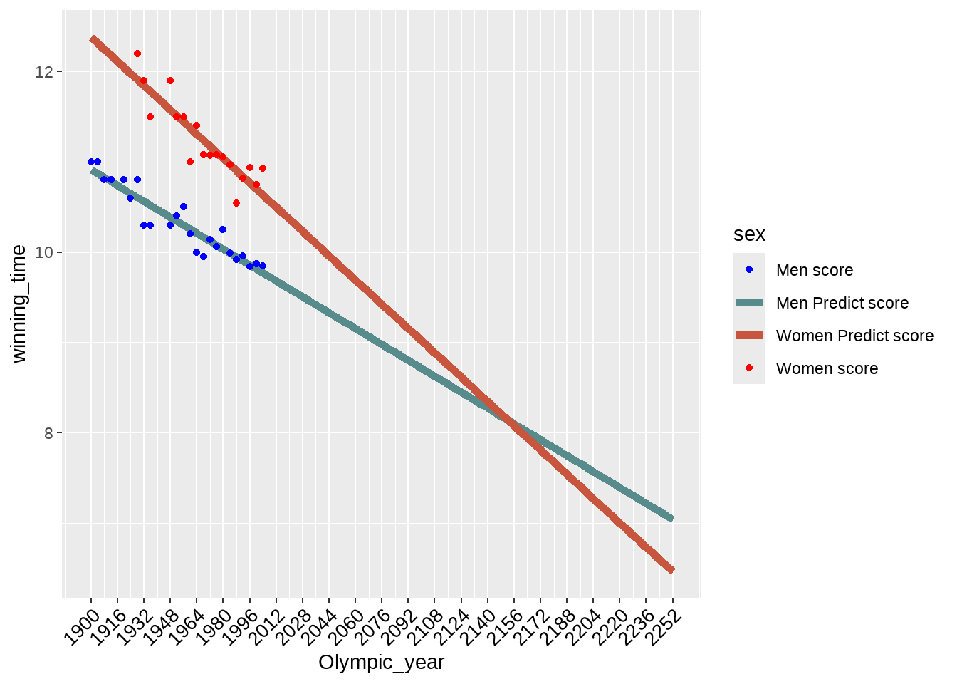 早知道nature文章这么简单,10年前我也可以写啊!
79.6 list_column
这里是另外的一种方法
d1 <- d %>%
  pivot_longer(
    cols = -Olympic_year,
    names_to = "sex",
    values_to = "winning_time"
  )

fit_model <- function(df) lm(winning_time ~ Olympic_year, data = df)

d2 <- d1 %>%
  group_nest(sex) %>%
  mutate(
    mod = map(data, fit_model)
  )
d2
## # A tibble: 2 × 3
## sex data mod
## <chr> <list<tibble[,2]>> <list>
## 1 Men_score [27 × 2] <lm>
## 2 Women_score [27 × 2] <lm>
# d2 %>% mutate(p = list(grid, grid))
# d3 <- d2 %>% mutate(p = list(grid, grid))
# d3
# d3 %>%
# mutate(
# predictions = map2(p, mod, add_predictions),
# )
# or
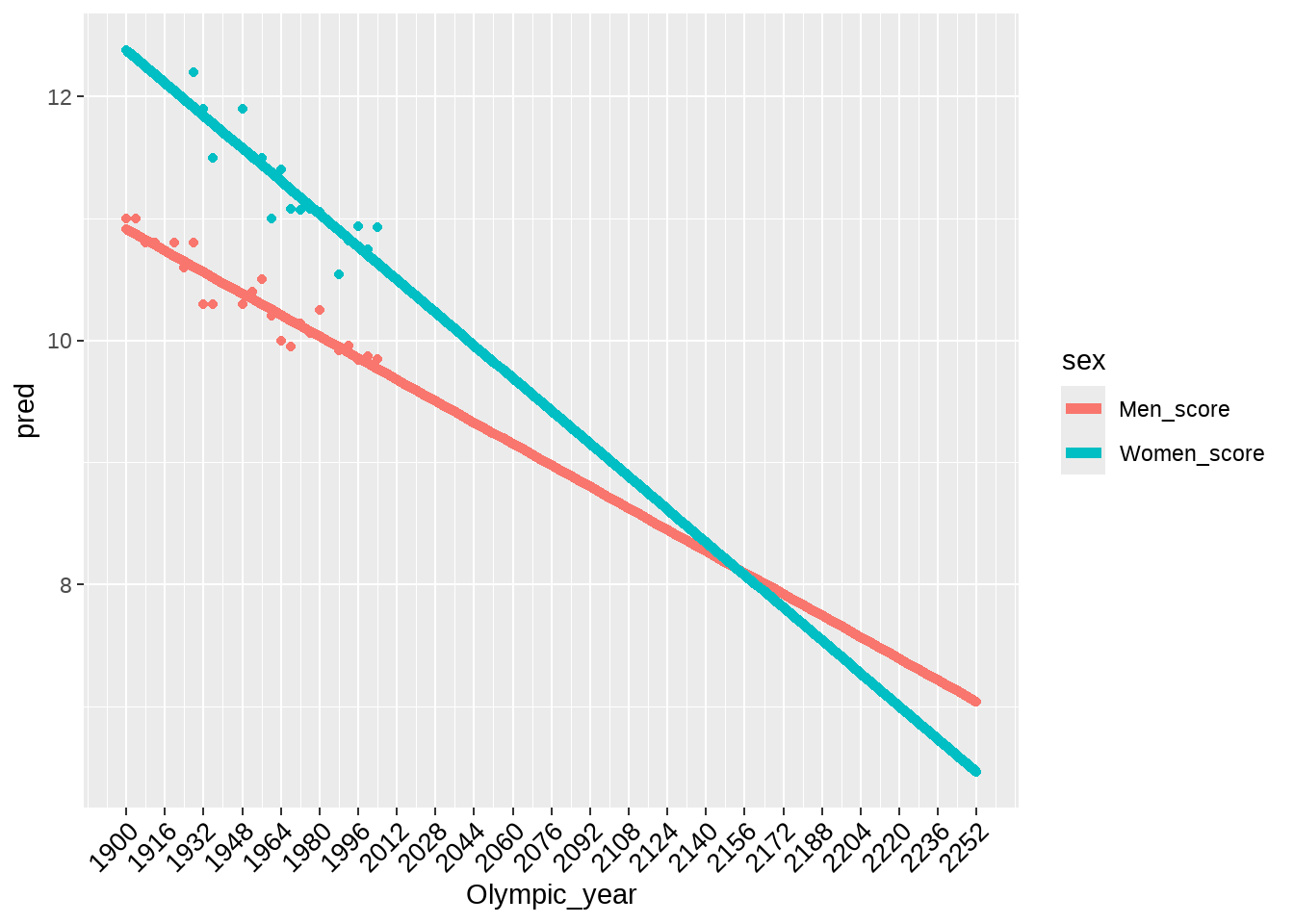
tb4 <- d2 %>%
mutate(
predictions = map(mod, ~ add_predictions(grid, .))
) %>%
select(sex, predictions) %>%
unnest(predictions)
tb4 %>%
ggplot(aes(
x = Olympic_year,
y = pred,
group = sex,
color = sex
)) +
geom_point() +
geom_line(size = 2) +
geom_point(
data = d1,
aes(
x = Olympic_year,
y = winning_time,
group = sex,
color = sex
)
) +
scale_x_continuous(
breaks = seq(1900, 2252, by = 16),
labels = as.character(seq(1900, 2252, by = 16))
) +
theme(axis.text.x = element_text(
size = 10, angle = 45, colour = "black",
vjust = 1, hjust = 1
))