第 82 章 探索性数据分析-身高体重
82.1 案例分析
这是一份身高和体重的数据集
## # A tibble: 10,000 × 3
##    Gender Height Weight
##    <chr>   <dbl>  <dbl>
##  1 Male     73.8   242.
##  2 Male     68.8   162.
##  3 Male     74.1   213.
##  4 Male     71.7   220.
##  5 Male     69.9   206.
##  6 Male     67.3   152.
##  7 Male     68.8   184.
##  8 Male     68.3   168.
##  9 Male     67.0   176.
## 10 Male     63.5   156.
## # ℹ 9,990 more rows## # A tibble: 1 × 3
## Gender Height Weight
## <int> <int> <int>
## 1 0 0 082.2 可视化
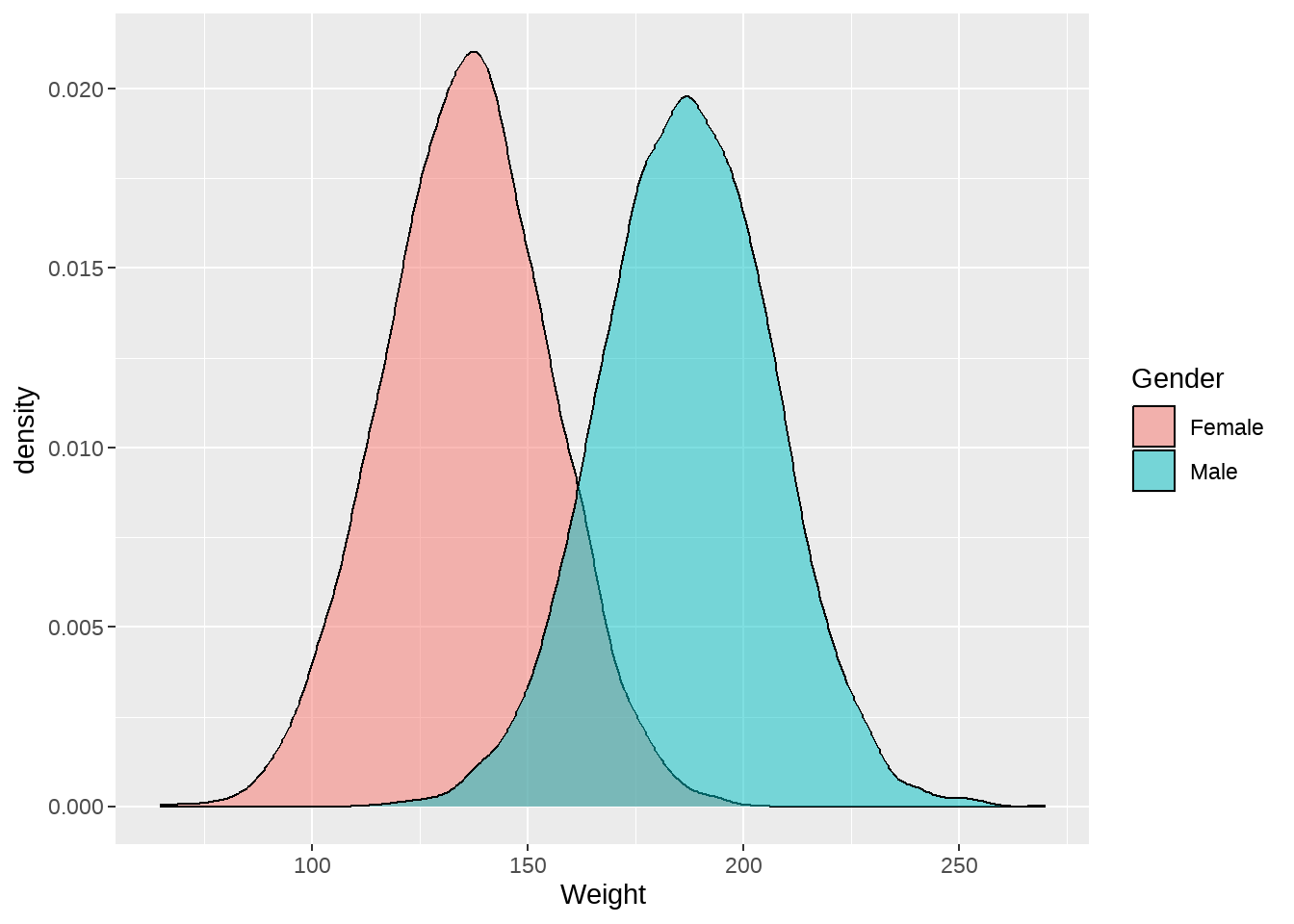
82.2.1 画出不同性别的身高分布
常规答案
d %>%
  ggplot(aes(x = Height, fill = Gender)) +
  geom_density(alpha = 0.5)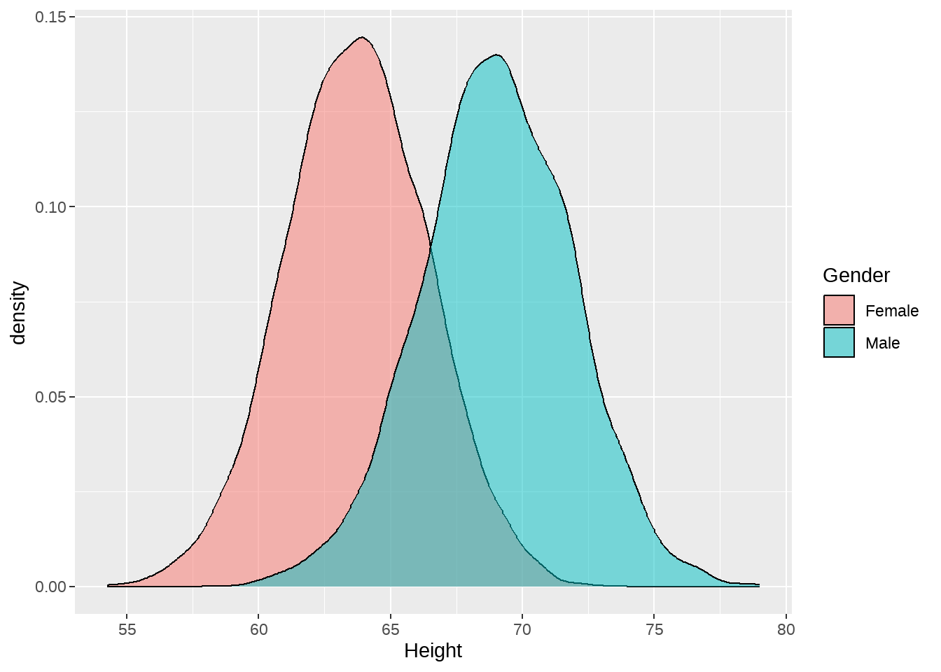
d %>%
  ggplot(aes(x = Height, fill = Gender)) +
  geom_density(alpha = 0.5) +
  facet_wrap(vars(Gender))
82.3 来点高级的
刚才我们看到了分面的操作,全局数据按照某个变量分组后,形成的若干个子集在不同的面板中分别展示出来。
这种方法很适合子集之间对比。事实上,我们看到每个子集的情况后,还很想知道全局的情况,以及子集在全局中的分布、状态或者位置。也就说,想对比子集和全局的情况。
所以我们期望(子集之间对比,子集与全局对比)。
具体方法:用分面的方法高亮展示子集,同时在每个分面上添加全局(灰色背景)
- 第一步,先把子集用分面的方法,分别画出来
d %>%
  ggplot(aes(x = Height)) +
  geom_density() +
facet_wrap(vars(Gender))- 第二步,添加整体的情况作为背景图层。因为第一步用到了分面,也就说会分组,但我们希望整体的背景图层不受分面信息影响,或者叫背景图层不需要分组,而是显示全部。也就说,要保证每个分面面板中的背景图都是一样的,因此,在这个geom_denstiy()图层中,构建不受facet_wrap()影响的数据,即删掉data的分组列。
d %>%
  ggplot(aes(x = Height)) +
  geom_density(
    data = d %>% select(-Gender)
  ) +
  geom_density() +
facet_wrap(vars(Gender))- 第三步,y轴的调整,我们希望保持密度的形状,同时希望y轴不用比例值而是用具体的count个数,这样整体和局部能放在一个标度下,
d %>%
  ggplot(aes(x = Height, y = after_stat(count))) +
  geom_density(
    data = d %>% select(-Gender)
  ) +
  geom_density() +
facet_wrap(vars(Gender))- 第四步, 配色。 配色网站选颜色
“Male”, “Female” 是Gender已经存在的分组。另外,我们在背景图层,新增了一个组”all people”,这样,整个图就有三个分组(三个color组),那么,我们可以在scale_fill_manual中统一设置和指定。
density_colors <- c(
  "Male" = "#247BA0",
  "Female" = "#F25F5C",
  "all people" = "grey85"
)
d %>%
  ggplot(aes(x = Height, y = after_stat(count))) +
  geom_density(
    data = df %>% select(-Gender),
    aes(fill = "all people", color = "all people")
  ) +
  geom_density(aes(color = Gender, fill = Gender)) +
  facet_wrap(vars(Gender)) +
  scale_fill_manual(name = NULL, values = density_colors) +
  scale_color_manual(name = NULL, values = density_colors) +
  theme_minimal() +
  theme(legend.position = "bottom")
82.3.1 完整代码
density_colors <- c(
  "Male" = "#247BA0",
  "Female" = "#F25F5C",
  "all people" = "grey80"
)

scales::show_col(density_colors)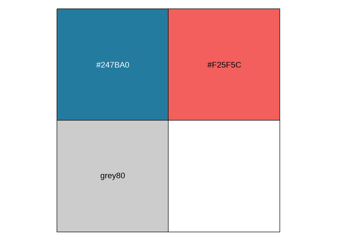
d %>%
  ggplot(aes(x = Height, y = after_stat(count))) +
  geom_density(
    data = d %>% dplyr::select(-Gender),
    aes(fill = "all people", color = "all people")
  ) +
  geom_density(aes(color = Gender, fill = Gender)) +
  facet_wrap(vars(Gender)) +
  scale_fill_manual(name = NULL, values = density_colors) +
  scale_color_manual(name = NULL, values = density_colors) +
  theme_minimal() +
  theme(legend.position = "bottom")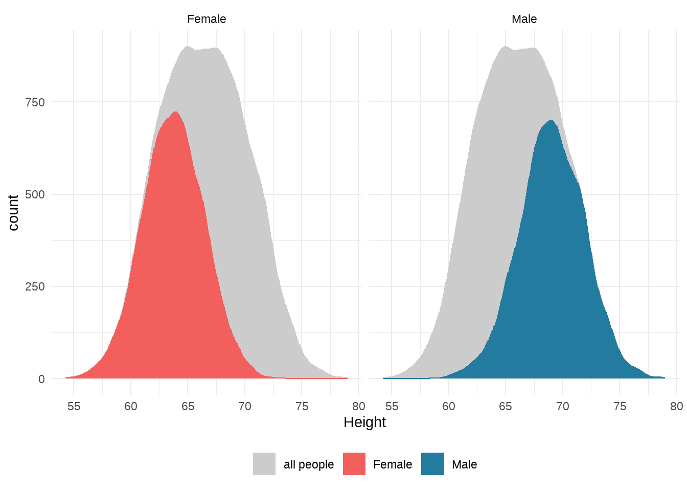
或者,用不同的主题风格
density_colors <- c(
  "Male" = "#56B4E9",
  "Female" = "#EF8A17",
  "all participants" = "grey85"
)

d %>%
  ggplot(aes(x = Height, y = after_stat(count))) +
  geom_density(
    data = function(x) dplyr::select(x, -Gender),
    aes(fill = "all participants", color = "all participants")
  ) +
  geom_density(aes(fill = Gender, color = Gender)) +
  facet_wrap(vars(Gender)) +
  scale_color_manual(name = NULL, values = density_colors) +
  scale_fill_manual(name = NULL, values = density_colors) +
  cowplot::theme_minimal_hgrid(16) +
  theme(legend.position = "bottom", legend.justification = "center")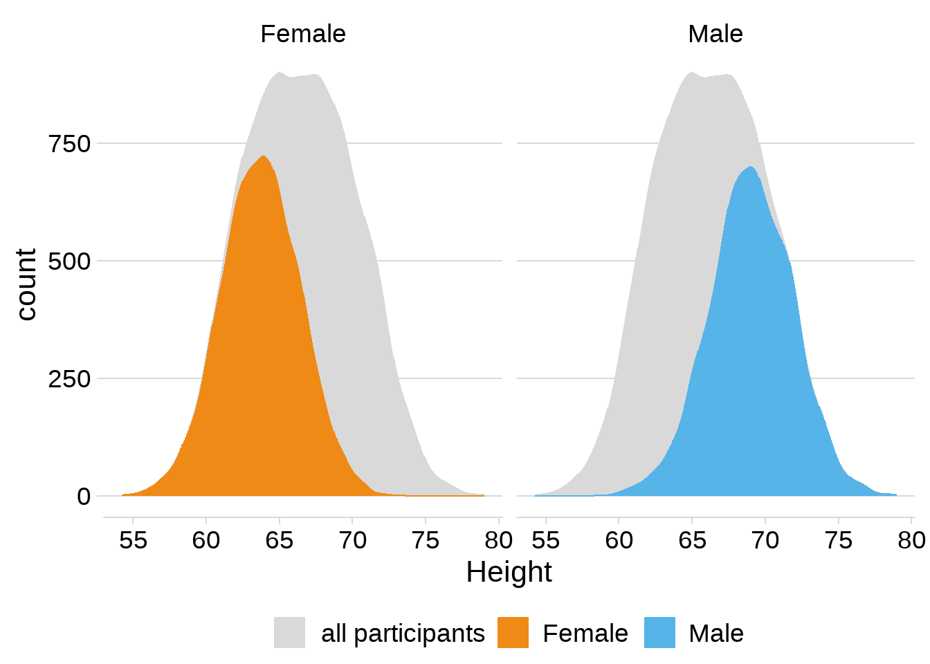
82.4 建模
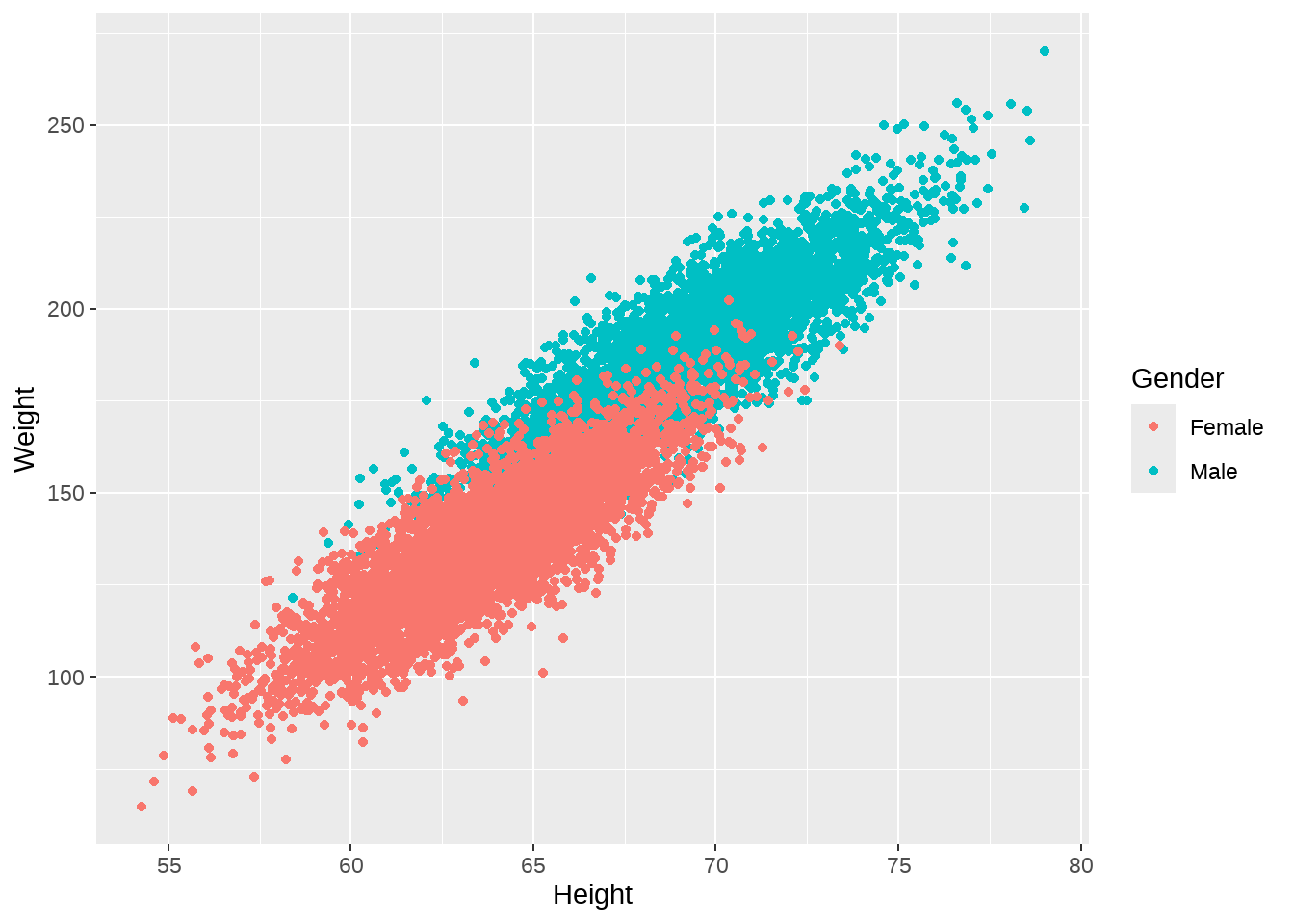
82.4.2 建立身高与体重的线性模型
##
## Call:
## lm(formula = Weight ~ 1 + Height, data = d)
##
## Residuals:
##     Min      1Q  Median      3Q     Max
## -51.934  -8.236  -0.119   8.260  46.844
##
## Coefficients:
##               Estimate Std. Error t value Pr(>|t|)
## (Intercept) -350.73719    2.11149  -166.1   <2e-16 ***
## Height         7.71729    0.03176   243.0   <2e-16 ***
## ---
## Signif. codes:  0 '***' 0.001 '**' 0.01 '*' 0.05 '.' 0.1 ' ' 1
##
## Residual standard error: 12.22 on 9998 degrees of freedom
## Multiple R-squared:  0.8552, Adjusted R-squared:  0.8552
## F-statistic: 5.904e+04 on 1 and 9998 DF,  p-value: < 2.2e-16
broom::tidy(fit)## # A tibble: 2 × 5
## term estimate std.error statistic p.value
## <chr> <dbl> <dbl> <dbl> <dbl>
## 1 (Intercept) -351. 2.11 -166. 0
## 2 Height 7.72 0.0318 243. 082.4.3 建立不同性别下的身高与体重的线性模型
## # A tibble: 4 × 6
## # Groups:   Gender [2]
##   Gender term        estimate std.error statistic p.value
##   <chr>  <chr>          <dbl>     <dbl>     <dbl>   <dbl>
## 1 Female (Intercept)  -246.      3.36       -73.3       0
## 2 Female Height          5.99    0.0526     114.        0
## 3 Male   (Intercept)  -224.      3.41       -65.8       0
## 4 Male   Height          5.96    0.0494     121.        0
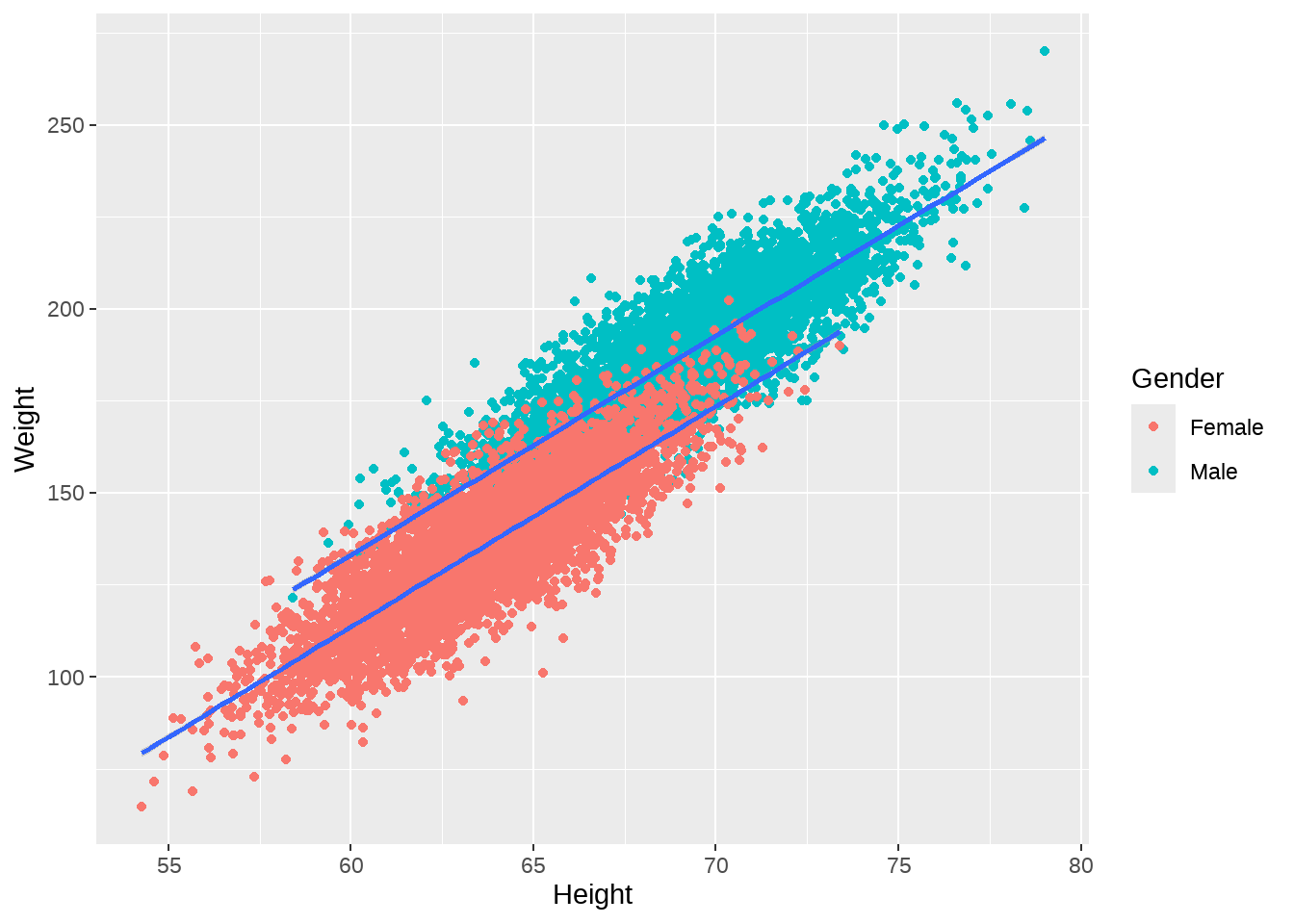
d %>%
  ggplot(aes(x = Height, y = Weight, group = Gender)) +
  geom_point(aes(color = Gender)) +
  geom_smooth(method = lm)