第 68 章 贝叶斯广义线性模型
library(tidyverse)
library(tidybayes)
library(rstan)
library(wesanderson)


rstan_options(auto_write = TRUE)
options(mc.cores = parallel::detectCores())

theme_set(
  bayesplot::theme_default() +
  ggthemes::theme_tufte() +
    theme(plot.background = element_rect(fill = wes_palette("Moonrise2")[3],
                                         color = wes_palette("Moonrise2")[3]))
)
68.1 广义线性模型
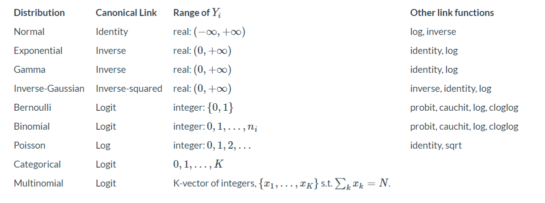
广义线性模型必须要明确的三个元素:
响应变量的概率分布(Normal, Binomial, Poisson, Categorical, Multinomial, Poisson, Beta)
预测变量的线性组合
\[ \eta = X \vec{\beta} \]
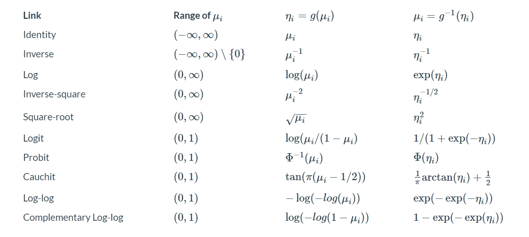
- 连接函数(\(g(.)\)), 将期望值映射到预测变量的线性组合 \[ g(\mu) = \eta \]
连接函数是可逆的(invertible)。连接函数的逆,将预测变量的线性组合映射到响应变量的期望值
\[ \mu = g^{-1}(\eta) \]
通过值域来看,连接函数的逆,将 \(\eta\) 从 \((-\infty, +\infty)\) 转换到特定的范围.
68.2 研究生院录取时有性别歧视?
这是美国一所大学研究生院的录取人数。我们想看下是否存在性别歧视?
UCBadmit <- readr::read_rds(here::here('demo_data', "UCBadmit.rds")) %>%
       mutate(applicant_gender = factor(applicant_gender, levels = c("male", "female")))
UCBadmit
## dept applicant_gender admit rejection applications ratio
## 1 A male 512 313 825 0.62060606
## 2 A female 89 19 108 0.82407407
## 3 B male 353 207 560 0.63035714
## 4 B female 17 8 25 0.68000000
## 5 C male 120 205 325 0.36923077
## 6 C female 202 391 593 0.34064081
## 7 D male 138 279 417 0.33093525
## 8 D female 131 244 375 0.34933333
## 9 E male 53 138 191 0.27748691
## 10 E female 94 299 393 0.23918575
## 11 F male 22 351 373 0.05898123
## 12 F female 24 317 341 0.07038123我们首先将申请者的性别作为预测变量,建立二项式回归模型如下
\[ \begin{align*} \text{admit}_i & \sim \operatorname{Binomial}(n_i, p_i) \\ \text{logit}(p_i) & = \alpha_{\text{gender}[i]} \\ \alpha_j & \sim \operatorname{Normal}(0, 1.5), \end{align*} \]
这里连接函数logit()需要说明一下
$$ \[\begin{align*} \text{logit}(p_{i}) &= \log\Big(\frac{p_{i}}{1 - p_{i}}\Big) = \alpha_{\text{gender}[i]}\\ \text{equivalent to,} \quad p_{i} &= \frac{1}{1 + \exp[- \alpha_{\text{gender}[i]}]} \\ & = \frac{\exp(\alpha_{\text{gender}[i]})}{1 + \exp (\alpha_{\text{gender}[i]})} \\ & = \text{inv_logit}(\alpha_{\text{gender}[i]}) \end{align*}\] $$
R语言glm函数能够拟合一系列的广义线性模型
model_logit <- glm(
  cbind(admit, rejection) ~ 0 + applicant_gender,
  data = UCBadmit,
  family = binomial(link = "logit")
)

summary(model_logit)
##
## Call:
## glm(formula = cbind(admit, rejection) ~ 0 + applicant_gender,
## family = binomial(link = "logit"), data = UCBadmit)
##
## Coefficients:
## Estimate Std. Error z value Pr(>|z|)
## applicant_gendermale -0.22013 0.03879 -5.675 1.38e-08 ***
## applicant_genderfemale -0.83049 0.05077 -16.357 < 2e-16 ***
## ---
## Signif. codes: 0 '***' 0.001 '**' 0.01 '*' 0.05 '.' 0.1 ' ' 1
##
## (Dispersion parameter for binomial family taken to be 1)
##
## Null deviance: 1107.08 on 12 degrees of freedom
## Residual deviance: 783.61 on 10 degrees of freedom
## AIC: 856.55
##
## Number of Fisher Scoring iterations: 468.2.1 Stan 代码
stan_program_A <- '
data {
  int n;
  int admit[n];
  int applications[n];
  int applicant_gender[n];
}
parameters {
  real a[2];
}
transformed parameters {
  vector[n] p;
  for (i in 1:n) {
    p[i] = inv_logit(a[applicant_gender[i]]);
  }
}
model {
  a ~ normal(0, 1.5);
  for (i in 1:n) {
    admit[i] ~ binomial(applications[i], p[i]);
  }
}
'

stan_data <- UCBadmit %>%
  compose_data()

fit01 <- stan(model_code = stan_program_A, data = stan_data)
fit01## Inference for Stan model: anon_model.
## 4 chains, each with iter=2000; warmup=1000; thin=1;
## post-warmup draws per chain=1000, total post-warmup draws=4000.
##
## mean se_mean sd 2.5% 25% 50% 75% 97.5% n_eff
## a[1] -0.22 0.00 0.04 -0.30 -0.25 -0.22 -0.19 -0.14 3964
## a[2] -0.83 0.00 0.05 -0.93 -0.86 -0.83 -0.80 -0.73 3792
## p[1] 0.45 0.00 0.01 0.43 0.44 0.45 0.45 0.46 3964
## p[2] 0.30 0.00 0.01 0.28 0.30 0.30 0.31 0.32 3790
## p[3] 0.45 0.00 0.01 0.43 0.44 0.45 0.45 0.46 3964
## p[4] 0.30 0.00 0.01 0.28 0.30 0.30 0.31 0.32 3790
## p[5] 0.45 0.00 0.01 0.43 0.44 0.45 0.45 0.46 3964
## p[6] 0.30 0.00 0.01 0.28 0.30 0.30 0.31 0.32 3790
## p[7] 0.45 0.00 0.01 0.43 0.44 0.45 0.45 0.46 3964
## p[8] 0.30 0.00 0.01 0.28 0.30 0.30 0.31 0.32 3790
## p[9] 0.45 0.00 0.01 0.43 0.44 0.45 0.45 0.46 3964
## p[10] 0.30 0.00 0.01 0.28 0.30 0.30 0.31 0.32 3790
## p[11] 0.45 0.00 0.01 0.43 0.44 0.45 0.45 0.46 3964
## p[12] 0.30 0.00 0.01 0.28 0.30 0.30 0.31 0.32 3790
## lp__ -2976.61 0.03 1.04 -2979.45 -2976.98 -2976.30 -2975.88 -2975.63 1551
## Rhat
## a[1] 1
## a[2] 1
## p[1] 1
## p[2] 1
## p[3] 1
## p[4] 1
## p[5] 1
## p[6] 1
## p[7] 1
## p[8] 1
## p[9] 1
## p[10] 1
## p[11] 1
## p[12] 1
## lp__ 1
##
## Samples were drawn using NUTS(diag_e) at Mon Oct 28 09:50:20 2024.
## For each parameter, n_eff is a crude measure of effective sample size,
## and Rhat is the potential scale reduction factor on split chains (at
## convergence, Rhat=1).
inv_logit <- function(x) {
  exp(x) / (1 + exp(x))
}


fit01 %>%
  tidybayes::spread_draws(a[i]) %>%
  pivot_wider(
    names_from = i,
    values_from = a,
    names_prefix = "a_"
  ) %>%
  mutate(
    diff_a = a_1 - a_2,
    diff_p = inv_logit(a_1) - inv_logit(a_2)
  ) %>%
  pivot_longer(contains("diff")) %>%
  group_by(name) %>%
  tidybayes::mean_qi(value, .width = .89)
## # A tibble: 2 × 7
## name value .lower .upper .width .point .interval
## <chr> <dbl> <dbl> <dbl> <dbl> <chr> <chr>
## 1 diff_a 0.610 0.508 0.710 0.89 mean qi
## 2 diff_p 0.141 0.119 0.164 0.89 mean qi从这个模型的结果看,男性确实有优势。
- 从 log-odd 度量看,男性录取率高于女性录取率
- 从概率的角度看,男性的录取概率比女性高 12% 到 16%
下面我们来看模型拟合的情况
fit01 %>%
  tidybayes::gather_draws(p[i]) %>%
  tidybayes::mean_qi(.width = .89) %>%
  ungroup() %>%
  rename(Estimate = .value) %>%
  bind_cols(UCBadmit) %>%

  ggplot(aes(x = applicant_gender, y = ratio)) +
  geom_point(aes(y = Estimate),
             color = wes_palette("Moonrise2")[1],
             shape = 1, size = 3
             ) +
  geom_point(color = wes_palette("Moonrise2")[2]) +
  geom_line(aes(group = dept),
            color = wes_palette("Moonrise2")[2]) +
  scale_y_continuous(limits = 0:1) +

  facet_grid(. ~ dept) +
  labs(x = NULL, y = 'Probability of admission')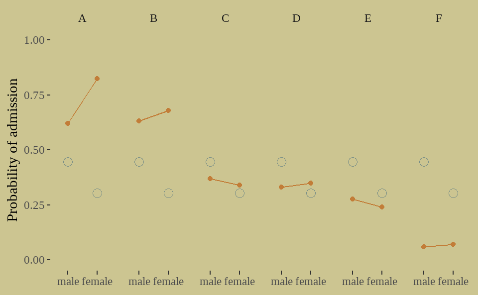
我们能说存在性别歧视?我们发现一些违反直觉的问题:
原始数据中只有学院C和E,女性录取率略低于男性,但模型结果却表明,女性预期的录取概率比男性低14%。
同时,我们看到男性和女性申请的院系不一样,以下是各学院男女申请人数的比例。女性更倾向与选择A、B之外的学院,比如F学院,而这些学院申请人数比较多,因而男女录取率都很低,甚至不到10%. 也就说,大多女性选择录取率低的学院,从而拉低了女性整体的录取率。
UCBadmit %>%
  group_by(dept) %>%
  mutate(proportion = applications / sum(applications)) %>%
  select(dept, applicant_gender, proportion) %>%
  pivot_wider(
    names_from = dept,
    values_from = proportion
  ) %>%
  mutate(
    across(where(is.double), round, digits = 2)
  )
## # A tibble: 2 × 7
## applicant_gender A B C D E F
## <fct> <dbl> <dbl> <dbl> <dbl> <dbl> <dbl>
## 1 male 0.88 0.96 0.35 0.53 0.33 0.52
## 2 female 0.12 0.04 0.65 0.47 0.67 0.48- 模型没有问题,而是我们的提问(对全体学院,男女平均录取率有什么差别?)是有问题的。
因此,我们的提问要修改为:在每个院系内部,男女平均录取率的差别是多少?
68.2.2 增加预测变量
增加院系项,也就说一个院系对应一个单独的截距,可以捕获院系之间的录取率差别。
\[ \begin{align*} \text{admit}_i & \sim \operatorname{Binomial} (n_i, p_i) \\ \text{logit}(p_i) & = \alpha_{\text{gender}[i]} + \delta_{\text{dept}[i]} \\ \alpha_j & \sim \operatorname{Normal} (0, 1.5) \\ \delta_k & \sim \operatorname{Normal} (0, 1.5), \end{align*} \]
stan_program_B <- '
data {
  int n;
  int n_dept;
  int admit[n];
  int applications[n];
  int applicant_gender[n];
  int dept[n];
}
parameters {
  real a[2];
  real b[n_dept];
}
transformed parameters {
  vector[n] p;
  for (i in 1:n) {
    p[i] = inv_logit(a[applicant_gender[i]] + b[dept[i]]);
  }
}
model {
  a ~ normal(0, 1.5);
  b ~ normal(0, 1.5);
  for (i in 1:n) {
    admit[i] ~ binomial(applications[i], p[i]);
  }
}
'
stan_data <- UCBadmit %>%
  compose_data()

fit02 <- stan(model_code = stan_program_B, data = stan_data)
fit02## Inference for Stan model: anon_model.
## 4 chains, each with iter=2000; warmup=1000; thin=1;
## post-warmup draws per chain=1000, total post-warmup draws=4000.
##
## mean se_mean sd 2.5% 25% 50% 75% 97.5% n_eff
## a[1] -0.48 0.03 0.50 -1.52 -0.81 -0.45 -0.17 0.46 390
## a[2] -0.39 0.03 0.51 -1.43 -0.71 -0.36 -0.07 0.56 394
## b[1] 1.06 0.03 0.51 0.09 0.75 1.04 1.39 2.10 394
## b[2] 1.02 0.03 0.51 0.06 0.70 1.00 1.36 2.06 400
## b[3] -0.20 0.03 0.51 -1.15 -0.52 -0.22 0.13 0.84 396
## b[4] -0.23 0.03 0.51 -1.19 -0.55 -0.25 0.10 0.83 397
## b[5] -0.67 0.03 0.51 -1.62 -1.00 -0.70 -0.33 0.37 400
## b[6] -2.23 0.03 0.52 -3.21 -2.56 -2.25 -1.89 -1.13 410
## p[1] 0.64 0.00 0.02 0.61 0.63 0.64 0.65 0.67 5023
## p[2] 0.66 0.00 0.02 0.62 0.65 0.66 0.68 0.70 4151
## p[3] 0.63 0.00 0.02 0.59 0.62 0.63 0.64 0.67 4757
## p[4] 0.65 0.00 0.03 0.60 0.63 0.65 0.67 0.70 3959
## p[5] 0.34 0.00 0.02 0.30 0.32 0.34 0.35 0.37 4677
## p[6] 0.36 0.00 0.02 0.32 0.35 0.36 0.37 0.39 5350
## p[7] 0.33 0.00 0.02 0.29 0.32 0.33 0.34 0.37 4410
## p[8] 0.35 0.00 0.02 0.31 0.34 0.35 0.36 0.39 4632
## p[9] 0.24 0.00 0.02 0.20 0.23 0.24 0.25 0.28 4224
## p[10] 0.26 0.00 0.02 0.22 0.25 0.26 0.27 0.30 4953
## p[11] 0.06 0.00 0.01 0.05 0.06 0.06 0.07 0.08 2550
## p[12] 0.07 0.00 0.01 0.05 0.06 0.07 0.08 0.09 2817
## lp__ -2599.51 0.05 1.99 -2604.13 -2600.59 -2599.22 -2598.06 -2596.57 1448
## Rhat
## a[1] 1.01
## a[2] 1.01
## b[1] 1.01
## b[2] 1.01
## b[3] 1.01
## b[4] 1.01
## b[5] 1.01
## b[6] 1.01
## p[1] 1.00
## p[2] 1.00
## p[3] 1.00
## p[4] 1.00
## p[5] 1.00
## p[6] 1.00
## p[7] 1.00
## p[8] 1.00
## p[9] 1.00
## p[10] 1.00
## p[11] 1.00
## p[12] 1.00
## lp__ 1.00
##
## Samples were drawn using NUTS(diag_e) at Mon Oct 28 09:50:56 2024.
## For each parameter, n_eff is a crude measure of effective sample size,
## and Rhat is the potential scale reduction factor on split chains (at
## convergence, Rhat=1).
inv_logit <- function(x) {
  exp(x) / (1 + exp(x))
}


fit02 %>%
  tidybayes::spread_draws(a[i]) %>%
  pivot_wider(
    names_from = i,
    values_from = a,
    names_prefix = "a_"
  ) %>%
  mutate(
    diff_a = a_1 - a_2,
    diff_p = inv_logit(a_1) - inv_logit(a_2)
  ) %>%
  pivot_longer(contains("diff")) %>%
  group_by(name) %>%
  tidybayes::mean_qi(value, .width = .89)
## # A tibble: 2 × 7
## name value .lower .upper .width .point .interval
## <chr> <dbl> <dbl> <dbl> <dbl> <chr> <chr>
## 1 diff_a -0.0982 -0.228 0.0321 0.89 mean qi
## 2 diff_p -0.0223 -0.0531 0.00706 0.89 mean qi从第二个模型的结果看,男性没有优势,甚至不如女性。
- 从 log-odd 度量看,男性录取率低于女性录取率
- 从概率的角度看,男性的录取概率比女性低 2%
(增加了一个变量,剧情反转了。辛普森佯谬)
fit02 %>%
  tidybayes::gather_draws(p[i]) %>%
  tidybayes::mean_qi(.width = .89) %>%
  ungroup() %>%
  rename(Estimate = .value) %>%
  bind_cols(UCBadmit) %>%

  ggplot(aes(x = applicant_gender, y = ratio)) +
  geom_point(aes(y = Estimate),
             color = wes_palette("Moonrise2")[1],
             shape = 1, size = 3
             ) +
  geom_point(color = wes_palette("Moonrise2")[2]) +
  geom_line(aes(group = dept),
            color = wes_palette("Moonrise2")[2]) +
  scale_y_continuous(limits = 0:1) +

  facet_grid(. ~ dept) +
  labs(x = NULL, y = 'Probability of admission')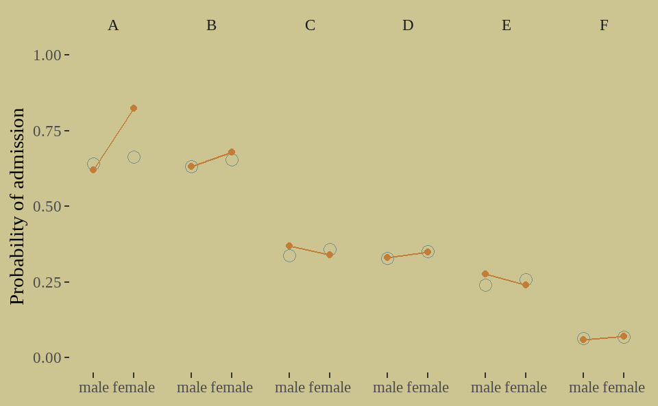
从图看出,我们第二个模型能够捕捉到数据大部分特征,但还有改进空间。
68.3 作业
讲性别从模型中去除,然后看看模型结果
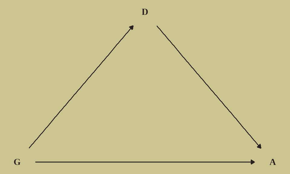
如果我们假定申请人性别影响院系选择和录取率,把院系当作中介,建立中介模型
library(ggdag)

dag_coords <-
  tibble(name = c("G", "D", "A"),
         x    = c(1, 2, 3),
         y    = c(1, 2, 1))

dagify(D ~ G,
       A ~ D + G,
       coords = dag_coords) %>%

  ggplot(aes(x = x, y = y, xend = xend, yend = yend)) +
  geom_dag_text(color = wes_palette("Moonrise2")[4], family = "serif") +
  geom_dag_edges(edge_color = wes_palette("Moonrise2")[4]) +
  scale_x_continuous(NULL, breaks = NULL) +
  scale_y_continuous(NULL, breaks = NULL)