第 49 章 模拟与抽样2
我很推崇infer基于模拟的假设检验。本节课的内容是用tidyverse技术重复infer过程,让统计分析透明。
library(tidyverse)
library(infer)

penguins <- palmerpenguins::penguins %>% drop_na()

penguins %>%
  specify(formula = bill_length_mm ~ sex) %>%
  hypothesize(null = "independence") %>%
  generate(reps = 5000, type = "permute") %>%
  calculate(
    stat = "diff in means",
    order = c("male", "female")
  ) %>%
  visualize()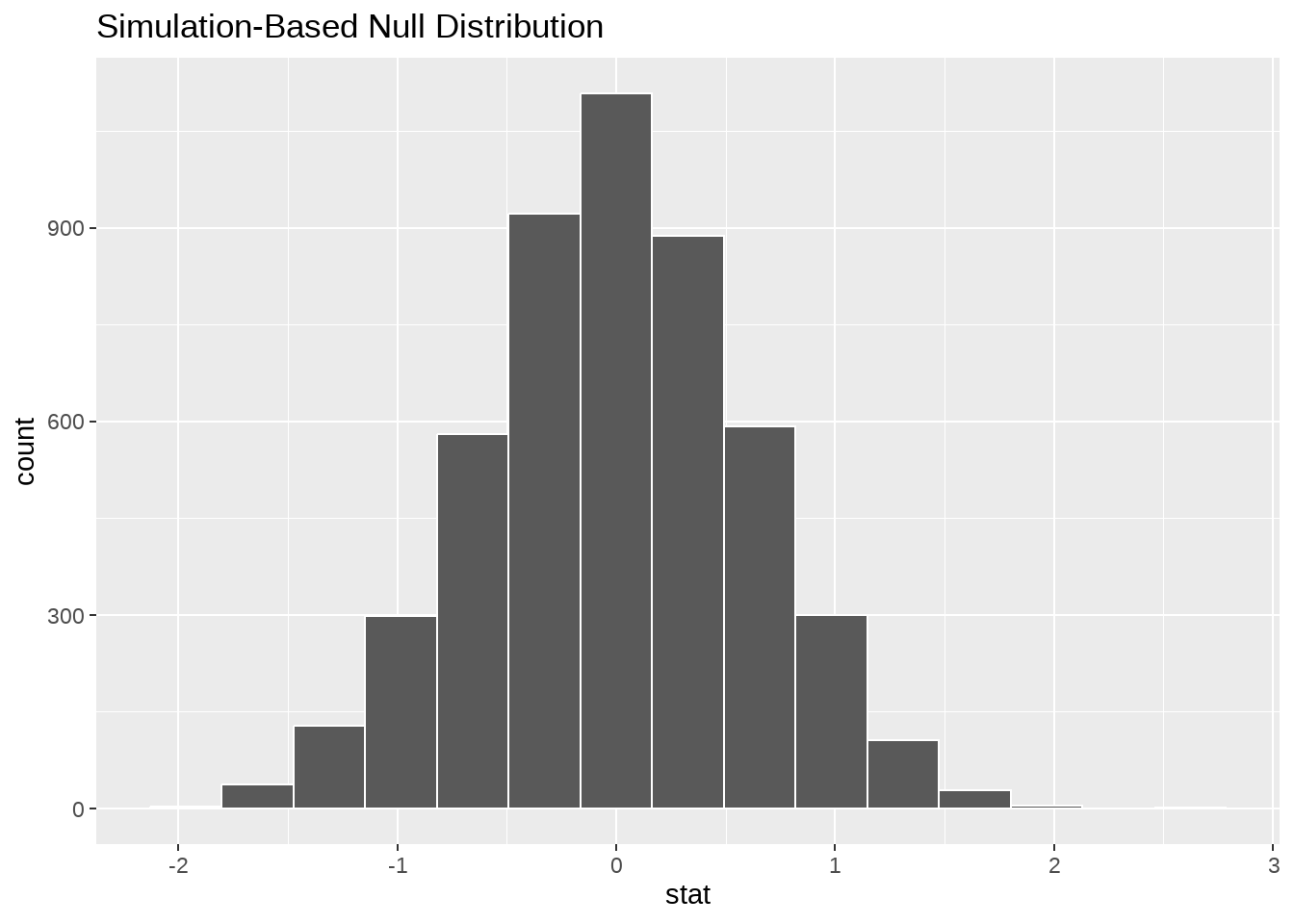
49.1 重复infer中diff in means的抽样过程
两个假设:
- 独立性假设。假设有 y 和 x 两者独立,即y 与 x 无关,一个怎么变,都不会影响另一个。
- 零假设,x下有两个组(male, female),每组对应的y的均值是相等的,均值之差为0.
具体怎么做呢?
49.1.1 抽样
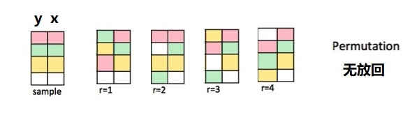
- 解释变量x列不动
- 响应变量y这一列,洗牌后放回。
相当于重新排列了y,所以抽样方法叫是”permute”。由图中可以看到每次抽样返回一个与原数据框大小相等的新数据框。下面以一个小的数据框为例演示
## # A tibble: 4 × 2
##       y x
##   <int> <chr>
## 1     1 a
## 2     2 a
## 3     3 b
## 4     4 b
重新排列y
## # A tibble: 4 × 2
##       y x
##   <int> <chr>
## 1     1 a
## 2     3 a
## 3     4 b
## 4     2 b
也可以写成函数形式
permute_once <- function(df) {
  y <- df[[1]]
  y_prime <- sample(y, size = length(y), replace = FALSE)

  df[1] <- y_prime
  return(df)
}

tbl %>% permute_once()
## # A tibble: 4 × 2
## y x
## <int> <chr>
## 1 3 a
## 2 4 a
## 3 2 b
## 4 1 b这个操作需要重复若干次,比如100次,即得到100个数据框,因此可以使用purrr::map()迭代
为方便灵活定义重复的次数,也可以改成函数,并且为每次返回的样本(数据框),编一个序号
permuate_repeat <- function(df, reps = 30){
  df_out <-
    purrr::map_dfr(.x = 1:reps, .f = ~ permute_once(df)) %>%
    dplyr::mutate(replicate = rep(1:reps, each = nrow(df))) %>%
    dplyr::group_by(replicate)

  return(df_out)
}

tbl %>% permuate_repeat(reps = 1000)
## # A tibble: 4,000 × 3
## # Groups: replicate [1,000]
## y x replicate
## <int> <chr> <int>
## 1 4 a 1
## 2 3 a 1
## 3 1 b 1
## 4 2 b 1
## 5 4 a 2
## 6 1 a 2
## 7 2 b 2
## 8 3 b 2
## 9 1 a 3
## 10 3 a 3
## # ℹ 3,990 more rows49.1.2 计算null假设分布
计算每次抽样中,a 组和 b 组的均值,以及这两个均值的差
null_dist <- tbl %>%
  permuate_repeat(reps = 1000) %>%

  group_by(replicate, x) %>%
  summarise(ybar = mean(y)) %>%
  group_by(replicate) %>%
  summarise(
    stat = ybar[x == "a"] - ybar[x == "b"]
  )

null_dist
## # A tibble: 1,000 × 2
## replicate stat
## <int> <dbl>
## 1 1 -2
## 2 2 1
## 3 3 -2
## 4 4 0
## 5 5 -1
## 6 6 0
## 7 7 1
## 8 8 -1
## 9 9 0
## 10 10 1
## # ℹ 990 more rows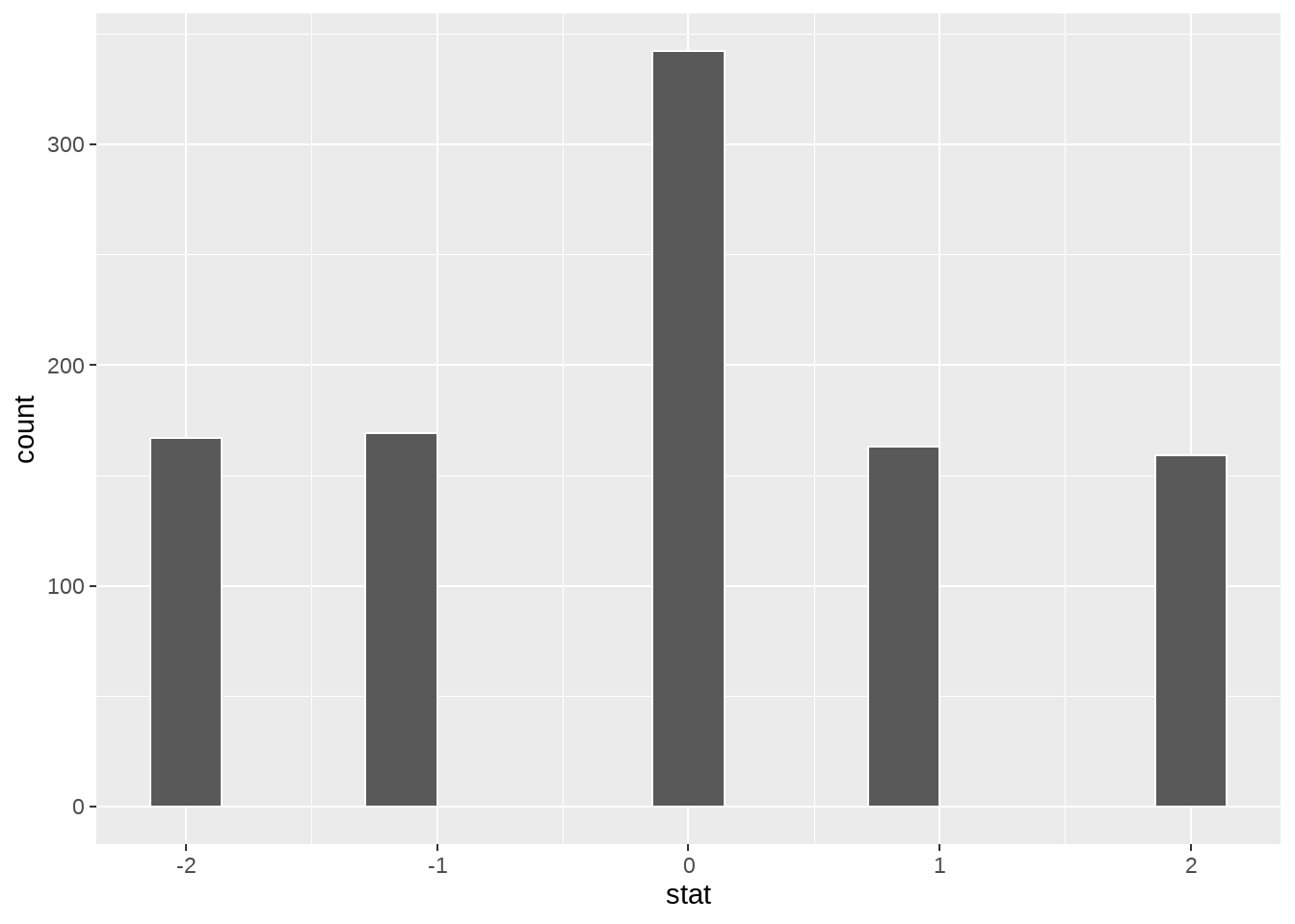
49.1.4 应用penguins
samples <- penguins %>%
select(bill_length_mm, sex) %>%
permuate_repeat(reps = 5000)
null_dist <- samples %>%
group_by(replicate, sex) %>%
summarise(ybar = mean(bill_length_mm)) %>%
group_by(replicate) %>%
summarise(
stat = ybar[sex == "male"] - ybar[sex == "female"]
)
null_dist %>%
  ggplot(aes(x = stat)) +
  geom_histogram(bins = 15, color = "white")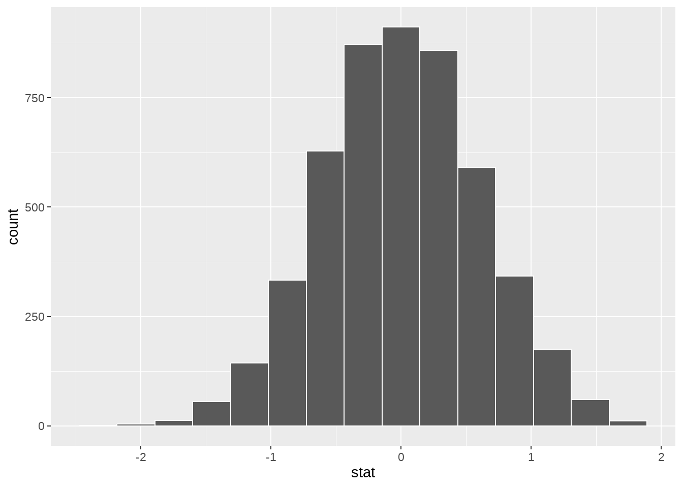
penguins %>%
  group_by(sex) %>%
  summarize(avg_rating = mean(bill_length_mm, na.rm = TRUE)) %>%
  mutate(diff_means = avg_rating - lag(avg_rating))
## # A tibble: 2 × 3
## sex avg_rating diff_means
## <fct> <dbl> <dbl>
## 1 female 42.1 NA
## 2 male 45.9 3.76## [1] 0