第 67 章 贝叶斯假设检验
library(tidyverse)
library(tidybayes)
library(rstan)

rstan_options(auto_write = TRUE)
options(mc.cores = parallel::detectCores())
theme_set(bayesplot::theme_default())
67.1 人们会给爱情片打高分?
这是一个关于电影评分的数据。我们想看下爱情片与动作片的平均得分是否存在显著不同?
## # A tibble: 100 × 5
##    title                          year rating genre  genre_numeric
##    <chr>                         <int>  <dbl> <fct>          <dbl>
##  1 One of Our Spies Is Missing    1966    5.6 Action             1
##  2 Black Pirate, The              1926    7.5 Action             1
##  3 Caged Heat 3000                1995    2.9 Action             1
##  4 G.P.U.                         1942    8.8 Action             1
##  5 Goal Club                      2001    9.2 Action             1
##  6 Dead or Alive: Hanzaisha       1999    6.9 Action             1
##  7 Lost in Africa                 1994    4   Action             1
##  8 Guns of the Magnificent Seven  1969    4.6 Action             1
##  9 Kiler                          1997    6.9 Action             1
## 10 Steamboy                       2004    6.6 Action             1
## # ℹ 90 more rows
67.1.1 可视化探索
看下两种题材电影评分的分布
movies %>%
  ggplot(aes(x = genre, y = rating, color = genre)) +
  geom_boxplot() +
  geom_jitter() +
  scale_x_discrete(
    expand = expansion(mult = c(0.5, 0.5))
  ) +
theme(legend.position = "none") 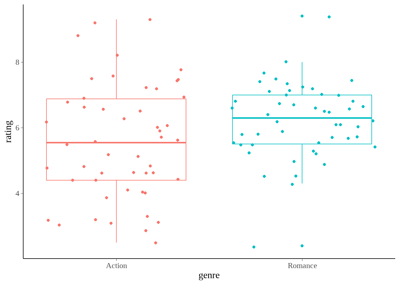
67.1.2 计算均值差
统计两种题材电影评分的均值
group_diffs <- movies %>%
  group_by(genre) %>%
  summarize(avg_rating = mean(rating, na.rm = TRUE)) %>%
  mutate(diff_means = avg_rating - lag(avg_rating))

group_diffs
## # A tibble: 2 × 3
## genre avg_rating diff_means
## <fct> <dbl> <dbl>
## 1 Action 5.55 NA
## 2 Romance 6.22 0.6767.1.3 t检验
传统的t检验
t.test(
  rating ~ genre,
  data = movies,
  var.equal = FALSE
)
##
## Welch Two Sample t-test
##
## data: rating by genre
## t = -2.2695, df = 83.737, p-value = 0.02581
## alternative hypothesis: true difference in means between group Action and group Romance is not equal to 0
## 95 percent confidence interval:
## -1.25709829 -0.08290171
## sample estimates:
## mean in group Action mean in group Romance
## 5.55 6.2267.2 stan 代码
67.2.1 normal分布
先假定rating评分,服从正态分布,同时不同的电影题材分组考虑
\[ \begin{aligned} \textrm{rating} & \sim \textrm{normal}(\mu_{\textrm{genre}}, \, \sigma _{\textrm{genre}}) \\ \mu &\sim \textrm{normal}(\textrm{mean_rating}, \, 2) \\ \sigma &\sim \textrm{cauchy}(0, \, 1) \end{aligned} \]
stan_program <- '
data {
  int<lower=1> N;
  int<lower=2> n_groups;
  vector[N] y;
  int<lower=1, upper=n_groups> group_id[N];
}
transformed data {
  real mean_y;
  mean_y = mean(y);
}
parameters {
  vector[2] mu;
  vector<lower=0>[2] sigma;
}
model {
  mu ~ normal(mean_y, 2);
  sigma ~ cauchy(0, 1);

  for (n in 1:N){
    y[n] ~ normal(mu[group_id[n]], sigma[group_id[n]]);
  }
}

generated quantities {
  real mu_diff;
  mu_diff = mu[2] - mu[1];
}

'

stan_data <- movies %>%
  select(genre, rating, genre_numeric) %>%
  tidybayes::compose_data(
    N        = nrow(.),
    n_groups = n_distinct(genre),
    group_id = genre_numeric,
    y        = rating
  )

stan_best_normal <- stan(model_code = stan_program, data = stan_data)
stan_best_normal## Inference for Stan model: anon_model.
## 4 chains, each with iter=2000; warmup=1000; thin=1;
## post-warmup draws per chain=1000, total post-warmup draws=4000.
##
## mean se_mean sd 2.5% 25% 50% 75% 97.5% n_eff Rhat
## mu[1] 5.55 0.00 0.25 5.06 5.39 5.55 5.72 6.07 4424 1
## mu[2] 6.22 0.00 0.16 5.91 6.12 6.22 6.33 6.54 3941 1
## sigma[1] 1.78 0.00 0.18 1.47 1.65 1.76 1.89 2.17 4042 1
## sigma[2] 1.15 0.00 0.12 0.95 1.06 1.13 1.22 1.41 3976 1
## mu_diff 0.67 0.00 0.30 0.07 0.46 0.67 0.87 1.25 4381 1
## lp__ -86.87 0.03 1.45 -90.42 -87.56 -86.52 -85.78 -85.08 2088 1
##
## Samples were drawn using NUTS(diag_e) at Mon Oct 28 09:48:29 2024.
## For each parameter, n_eff is a crude measure of effective sample size,
## and Rhat is the potential scale reduction factor on split chains (at
## convergence, Rhat=1).
stan_best_normal %>%
  tidybayes::spread_draws(mu_diff) %>%
  ggplot(aes(x = mu_diff)) +
  tidybayes::stat_halfeye() +
  geom_vline(xintercept = 0)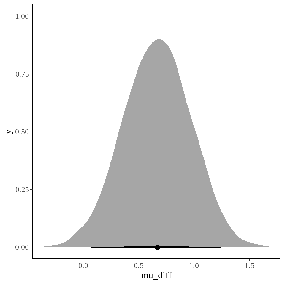
stan_best_normal %>%
  tidybayes::spread_draws(mu_diff) %>%

    ggplot(aes(x = mu_diff)) +
  stat_eye(side = "right",
           fill = "skyblue",
             point_interval = mode_hdi,
             .width = c(0.5, 0.89),
             interval_colour = "red",
             point_colour = "red",
             width = 15.5,
             height = 0.1
             ) +
  geom_vline(xintercept = c(-0.1, 0.1), linetype = "dashed", size = 1) +

  coord_cartesian(xlim = c(-1, 2)) +
    labs(x = "mu_diff", y = NULL)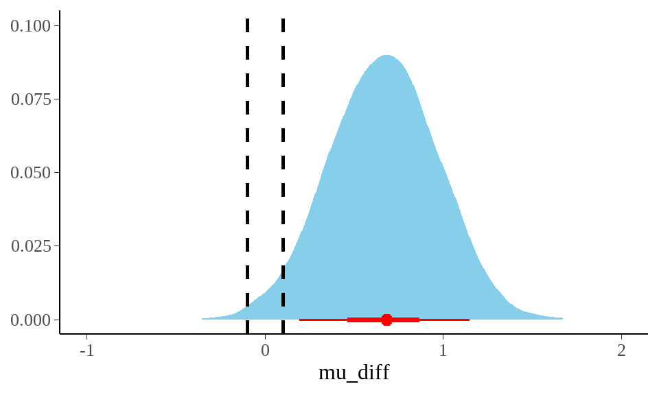
67.2.2 等效检验
我们一般会采用实用等效区间 region of practical equivalence ROPE。实用等效区间,就是我们感兴趣值附近的一个区间,比如这里的均值差。频率学中的零假设是看均值差是否为0,贝叶斯则是看均值差有多少落入0附近的区间。具体方法就是,先算出后验分布的高密度区间,然后看这个高密度区间落在[-0.1, 0.1]的比例.
lower <- -0.1*sd(movies$rating)
upper <-  0.1*sd(movies$rating)

stan_best_normal %>%
  tidybayes::spread_draws(mu_diff) %>%
  filter(
    mu_diff > ggdist::mean_hdi(mu_diff, .width = c(0.89))$ymin,
    mu_diff < ggdist::mean_hdi(mu_diff, .width = c(0.89))$ymax
  ) %>%
  summarise(
    percentage_in_rope = mean(between(mu_diff, lower, upper))
  )
## # A tibble: 1 × 1
## percentage_in_rope
## <dbl>
## 1 0在做假设检验的时候,我们内心是期望,后验概率的高密度区间落在实际等效区间的比例越小越小,如果小于2.5%,我们就可以拒绝零假设了;如果大于97.5%,我们就接受零假设。
stan_best_normal %>%
  tidybayes::spread_draws(mu_diff) %>%
  pull(mu_diff) %>%
  bayestestR::rope(x,
    range = c(-0.1, 0.1)*sd(movies$rating),
    ci = 0.89,
    ci_method = "HDI"
  )
## # Proportion of samples inside the ROPE [-0.15, 0.15]:
##
## inside ROPE
## -----------
## 0.00 %67.2.3 Student-t 分布
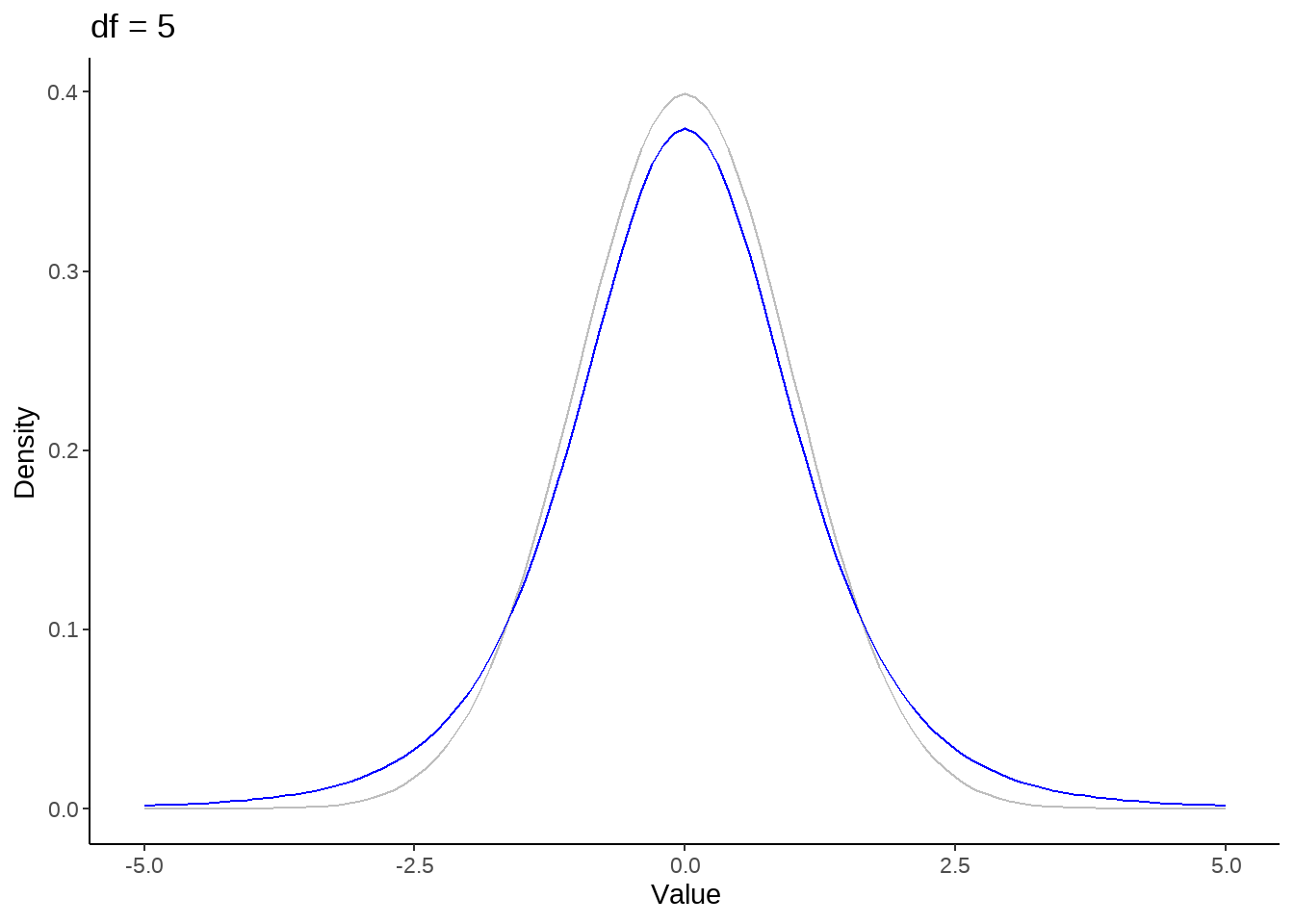
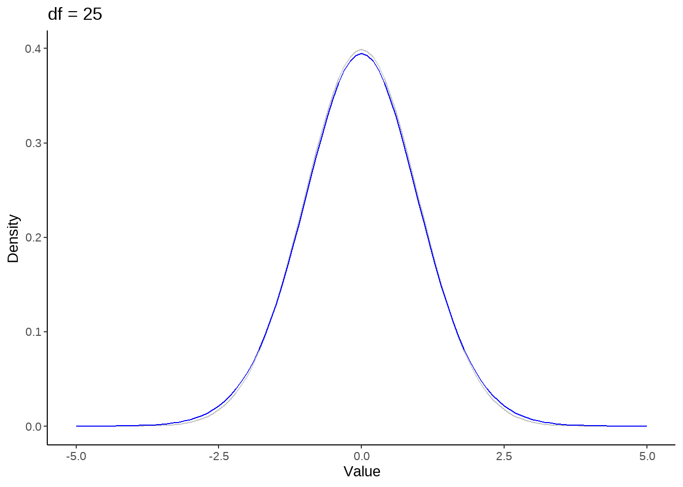
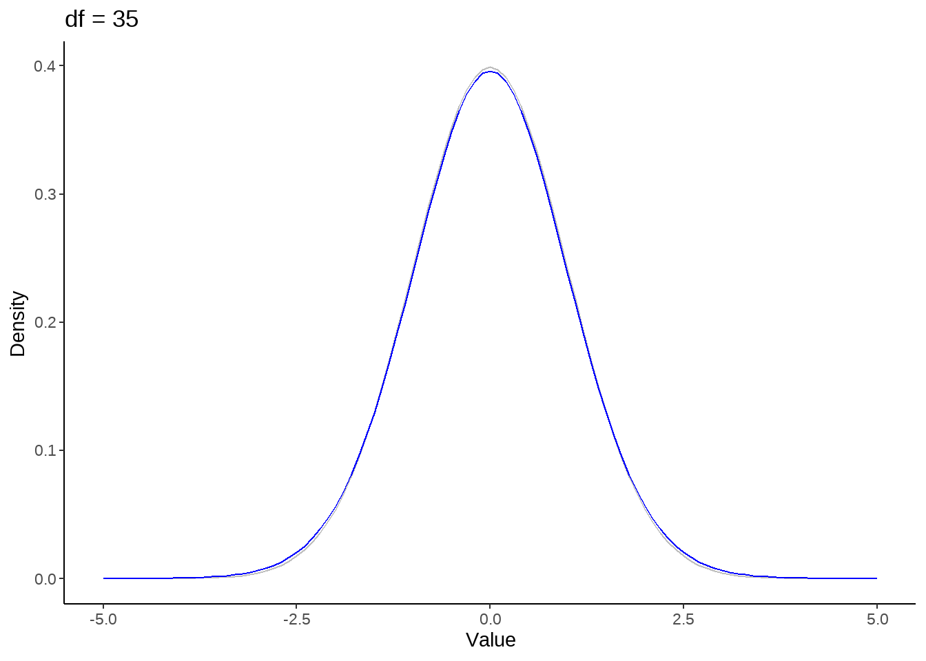
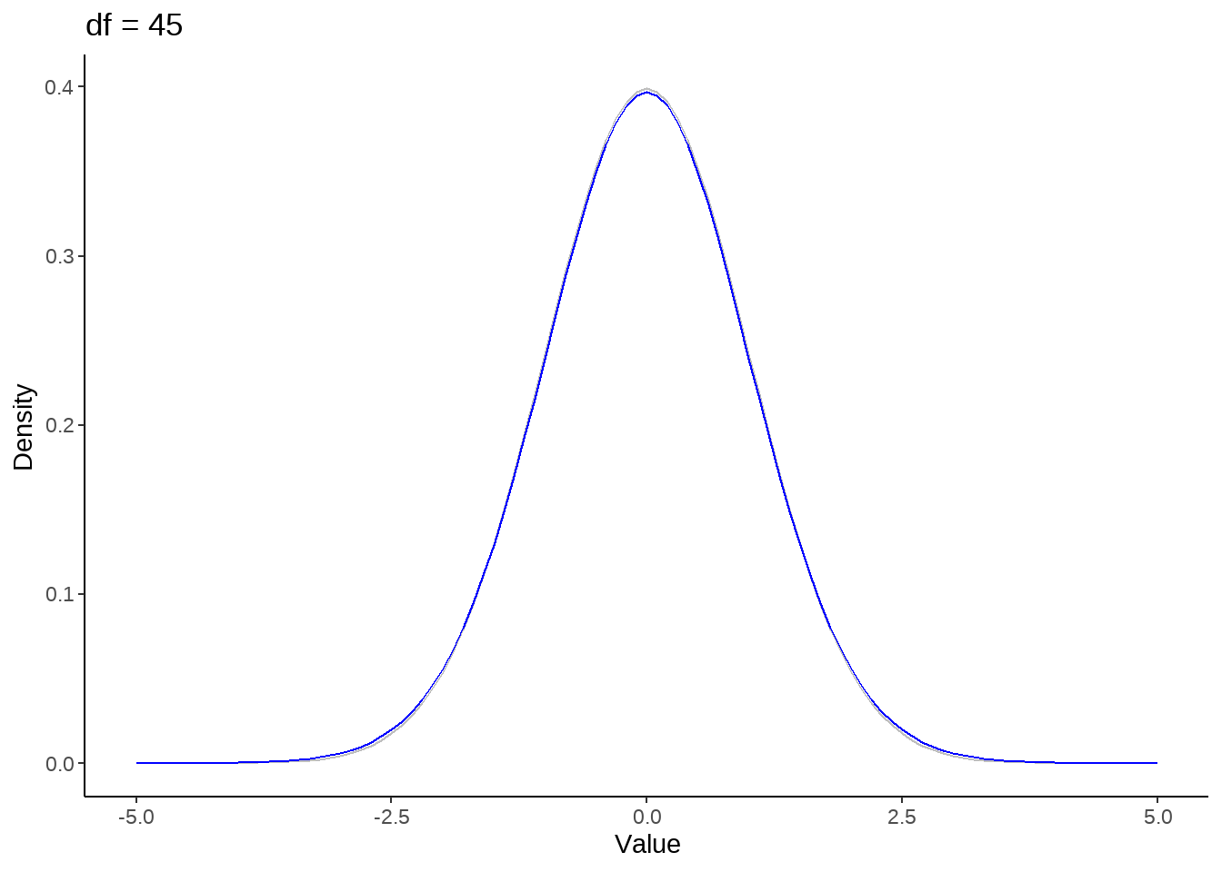
标准正态分布是t分布的极限分布
for (nu in c(1, seq(5, 50, by = 10))) {
 p <- tibble(x = seq(-5, 5, by=0.1)) %>%
    ggplot(aes(x)) +
    stat_function(fun = dnorm, color = 'gray') +
    stat_function(fun = dt, args = list(df = nu), color = 'blue') +
    theme_classic() +
    ylab("Density") +
    xlab('Value') +
    ggtitle(paste("df =", nu))

  print(p)
}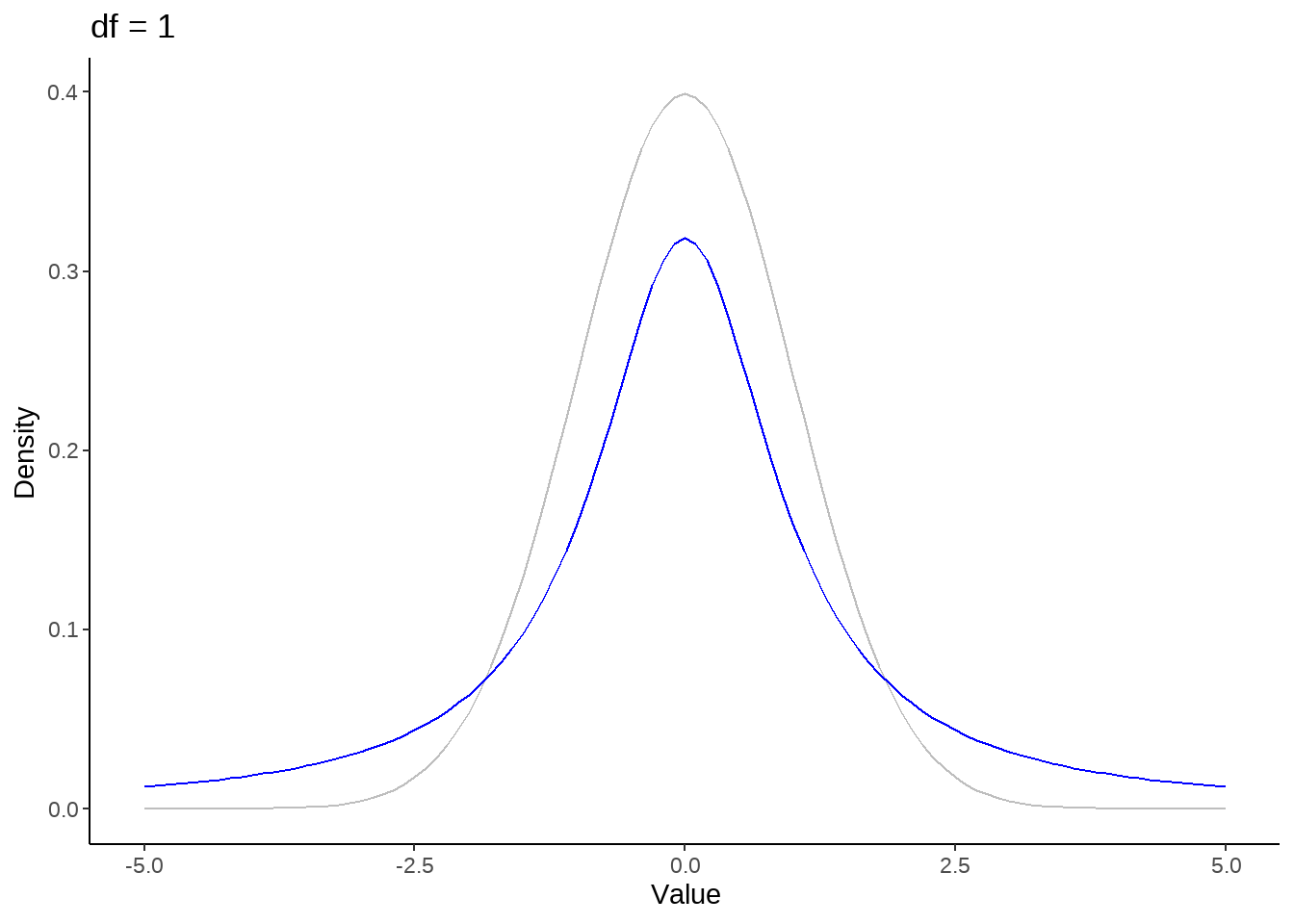

假定rating评分服从student-t分布,
\[ \begin{aligned} \textrm{rating} & \sim \textrm{student_t}(\nu, \,\mu_{\textrm{genre}}, \, \sigma _{\textrm{genre}}) \\ \mu &\sim \textrm{normal}(\textrm{mean_rating}, \, 2) \\ \sigma &\sim \textrm{cauchy}(0, \, 1) \\ \nu &\sim \textrm{exponential}(1.0/29) \end{aligned} \]
stan_program <- '
data {
  int<lower=1> N;
  int<lower=2> n_groups;
  vector[N] y;
  int<lower=1, upper=n_groups> group_id[N];
}
transformed data {
  real mean_y;
  mean_y = mean(y);
}
parameters {
  vector[2] mu;
  vector<lower=0>[2] sigma;
  real<lower=0, upper=100> nu;
}
model {
  mu ~ normal(mean_y, 2);
  sigma ~ cauchy(0, 1);
  nu ~ exponential(1.0/29);

  for (n in 1:N){
    y[n] ~ student_t(nu, mu[group_id[n]], sigma[group_id[n]]);
  }
}

generated quantities {
  real mu_diff;
  mu_diff = mu[2] - mu[1];
}

'

stan_data <- movies %>%
  select(genre, rating, genre_numeric) %>%
  tidybayes::compose_data(
    N        = nrow(.),
    n_groups = n_distinct(genre),
    group_id = genre_numeric,
    y        = rating
  )

stan_best_student <- stan(model_code = stan_program, data = stan_data)
stan_best_student## Inference for Stan model: anon_model.
## 4 chains, each with iter=2000; warmup=1000; thin=1;
## post-warmup draws per chain=1000, total post-warmup draws=4000.
##
## mean se_mean sd 2.5% 25% 50% 75% 97.5% n_eff
## mu[1] 5.53 0.00 0.25 5.04 5.37 5.53 5.70 6.01 4594
## mu[2] 6.24 0.00 0.15 5.93 6.13 6.24 6.34 6.54 3886
## sigma[1] 1.71 0.00 0.19 1.37 1.58 1.70 1.82 2.09 4167
## sigma[2] 1.05 0.00 0.13 0.81 0.97 1.05 1.13 1.33 2827
## nu 27.63 0.41 20.04 5.47 12.37 21.12 37.37 79.93 2434
## mu_diff 0.70 0.00 0.30 0.13 0.50 0.71 0.90 1.28 4224
## lp__ -119.46 0.04 1.66 -123.71 -120.27 -119.11 -118.24 -117.36 1733
## Rhat
## mu[1] 1
## mu[2] 1
## sigma[1] 1
## sigma[2] 1
## nu 1
## mu_diff 1
## lp__ 1
##
## Samples were drawn using NUTS(diag_e) at Mon Oct 28 09:49:08 2024.
## For each parameter, n_eff is a crude measure of effective sample size,
## and Rhat is the potential scale reduction factor on split chains (at
## convergence, Rhat=1).
stan_best_student %>%
  tidybayes::spread_draws(mu_diff) %>%
  ggplot(aes(x = mu_diff)) +
  tidybayes::stat_halfeye() +
  geom_vline(xintercept = 0)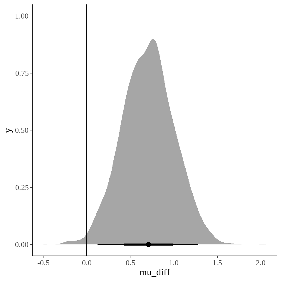
stan_best_student %>%
  as.data.frame() %>%
  head()
## mu[1] mu[2] sigma[1] sigma[2] nu mu_diff lp__
## 1 5.673473 6.149610 1.568025 1.166477 90.30934 0.47613707 -121.1445
## 2 5.504635 5.940376 1.585149 1.039357 71.98467 0.43574095 -121.0510
## 3 5.394744 5.876411 1.700437 1.043084 48.40776 0.48166637 -120.6530
## 4 5.873506 5.917845 1.855189 1.070505 44.63273 0.04433928 -120.6466
## 5 5.636965 6.297277 1.718054 1.079741 48.84739 0.66031242 -117.8778
## 6 5.271557 6.365048 1.888213 1.217796 17.65678 1.09349067 -119.5506
stan_best_student %>%
  as.data.frame() %>%
  ggplot(aes(x = `mu[1]`)) +
  geom_density()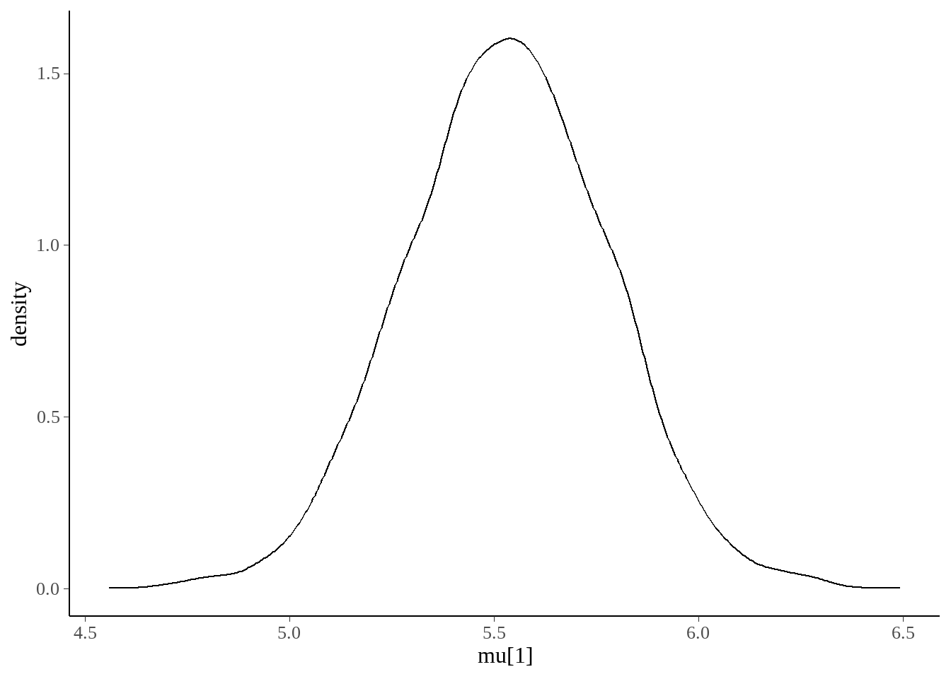
stan_best_student %>%
  tidybayes::gather_draws(mu[i], sigma[i]) %>%
  tidybayes::mean_hdi(.width = 0.89)
## # A tibble: 4 × 8
## i .variable .value .lower .upper .width .point .interval
## <int> <chr> <dbl> <dbl> <dbl> <dbl> <chr> <chr>
## 1 1 mu 5.53 5.13 5.91 0.89 mean hdi
## 2 1 sigma 1.71 1.40 1.98 0.89 mean hdi
## 3 2 mu 6.24 6.00 6.49 0.89 mean hdi
## 4 2 sigma 1.05 0.840 1.25 0.89 mean hdi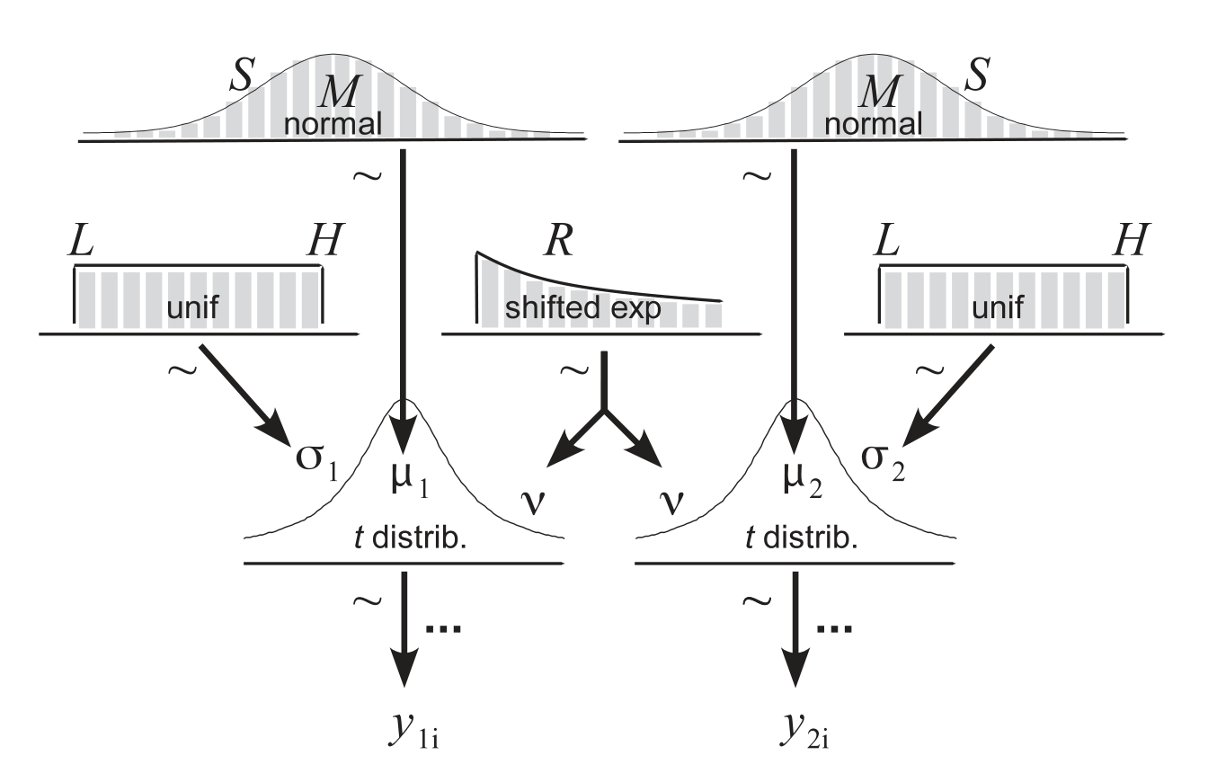
67.4 作业
- 将上一章线性模型的stan代码应用到电影评分数据中
\[ \begin{aligned} \textrm{rating} & \sim \textrm{Normal}(\mu, \, \sigma) \\ \mu & = \alpha + \beta \, \textrm{genre} \\ \alpha &\sim \textrm{Normal}(0, \, 5) \\ \beta &\sim \textrm{Normal}(0, \, 1) \\ \sigma &\sim \textrm{Exponential}(1) \\ \end{aligned} \]
stan_program <- '
data {
  int<lower=1> N;
  vector[N] y;
  vector[N] x;
}
parameters {
  real<lower=0> sigma;
  real alpha;
  real beta;
}

model {
  y ~ normal(alpha + beta * x, sigma);

  alpha ~ normal(0, 5);
  beta ~ normal(0, 1);
  sigma ~ exponential(1);
}

'

stan_data <- list(
    N   = nrow(movies),
    x   = as.numeric(movies$genre),
    y   = movies$rating
  )

stan_linear <- stan(model_code = stan_program, data = stan_data)
stan_linear## Inference for Stan model: anon_model.
## 4 chains, each with iter=2000; warmup=1000; thin=1;
## post-warmup draws per chain=1000, total post-warmup draws=4000.
##
## mean se_mean sd 2.5% 25% 50% 75% 97.5% n_eff Rhat
## sigma 1.48 0.00 0.11 1.30 1.41 1.48 1.55 1.71 2017 1
## alpha 4.91 0.01 0.47 4.00 4.60 4.91 5.23 5.80 1451 1
## beta 0.65 0.01 0.29 0.09 0.45 0.65 0.85 1.22 1482 1
## lp__ -91.25 0.03 1.22 -94.41 -91.80 -90.95 -90.34 -89.82 1306 1
##
## Samples were drawn using NUTS(diag_e) at Mon Oct 28 09:49:43 2024.
## For each parameter, n_eff is a crude measure of effective sample size,
## and Rhat is the potential scale reduction factor on split chains (at
## convergence, Rhat=1).
stan_linear %>%
  tidybayes::spread_draws(beta) %>%
  ggplot(aes(x = beta)) +
  tidybayes::stat_halfeye() +
  geom_vline(xintercept = 0)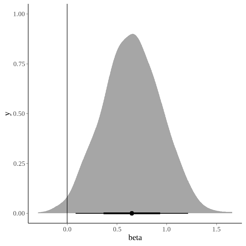
stan_linear %>%
  tidybayes::gather_draws(beta) %>%
  tidybayes::mean_hdi(.width = 0.89)
## # A tibble: 1 × 7
## .variable .value .lower .upper .width .point .interval
## <chr> <dbl> <dbl> <dbl> <dbl> <chr> <chr>
## 1 beta 0.649 0.178 1.13 0.89 mean hdi