第 29 章 ggplot2之数据可视化中的配色
为了让图更好看,需要在画图中使用配色,但如果从颜色的色相、色度、明亮度三个属性(Hue-Chroma-Luminance )开始学,感觉这样要学的东西太多了 😞. 事实上,大神们已经为我们准备好了很多好看的模板,我们可以偷懒直接拿来用🎵.
我个人比较喜欢colorspace中的配色,今天我们就讲讲如何使用这个宏包!
colorspace 宏包提供了三种类型的配色模板:
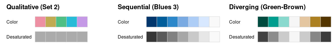
- Qualitative: 分类,用于呈现分类信息,比如不同种类用不同的颜色,颜色之间一般对比鲜明。
- Sequential: 序列,用于呈现有序/连续的数值信息,比如为了展示某地区黑人比例,比例越高颜色越深,比例越低颜色越浅。
- Diverging: 分歧,用于呈现有序/连续的数值信息,这些数值围绕着一个中心值,比中心值越大的方向用一种渐变色,比中心值越小用另一种渐变色。
三种类型对应着三个函数 qualitative_hcl(), sequential_hcl(), 和 diverging_hcl().
29.1 配色模板
根据你需要颜色的三大种类,先找适合的模板palettes
hcl_palettes(plot = TRUE)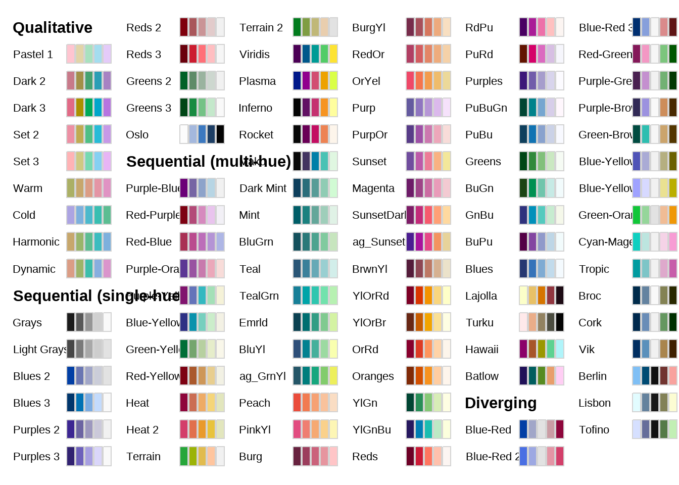
或者指定某个种类,显示所有的模板
hcl_palettes("qualitative", plot = TRUE)
hcl_palettes("sequential (single-hue)", n = 7, plot = TRUE)
hcl_palettes("sequential (multi-hue)", n = 7, plot = TRUE)
hcl_palettes("diverging", n = 7, plot = TRUE)
如果看中某个模板的颜色,可以获取它的值,比如sequential种类下的 “Peach”模板,
#colorspace::diverging_hcl(n = 7, "Dark 2")
#colorspace::qualitative_hcl(4, palette = "myset")
colorspace::sequential_hcl(n = 7, palette = "Peach")
## [1] "#EA4C3B" "#EF6D48" "#F3885B" "#F6A173" "#F8B78E" "#F9CCA9" "#FADDC3"当然,在用之前,我们先检验下
colorspace::sequential_hcl(n = 7, palette = "Peach") %>%
  colorspace::swatchplot()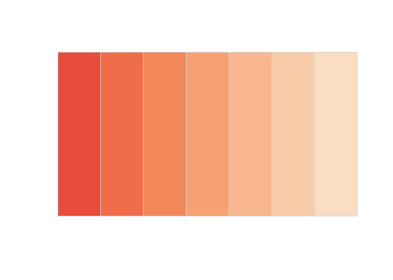
29.2 在ggplot2中使用
在ggplot2中可以免去手工操作,而直接使用。事实上,
colorspace 模板使用起来很方便,有统一格式scale_<aesthetic>_<datatype>_<colorscale>(),
- 这里
<aesthetic>是指定映射 (fill,color,colour), - 这里
<datatype>是表明数据变量的类型 (discrete,continuous,binned), - 这里
colorscale是声明颜色标度类型 (qualitative,sequential,diverging,divergingx).
| Scale function | Aesthetic | Data type | Palette type |
|---|---|---|---|
scale_color_discrete_qualitative() |
color |
discrete | qualitative |
scale_fill_continuous_sequential() |
fill |
continuous | sequential |
scale_colour_continuous_divergingx() |
colour |
continuous | diverging |
29.3 使用案例1
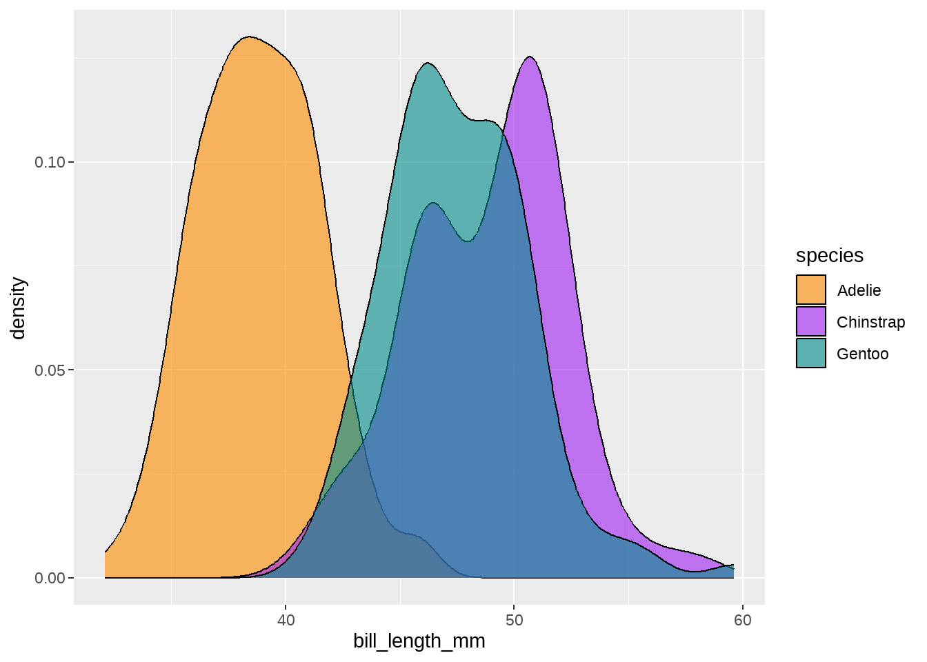
ggplot2默认
penguins %>%
   ggplot(aes(bill_length_mm, fill = species)) +
   geom_density(alpha = 0.6)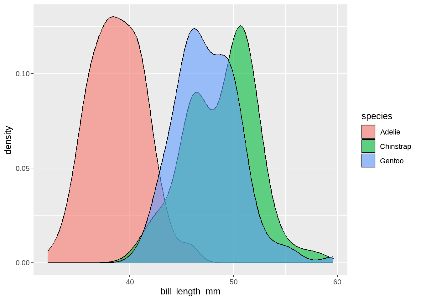
手动修改
penguins %>%
   ggplot(aes(bill_length_mm, fill = species)) +
   geom_density(alpha = 0.6) +
   scale_fill_manual(
     breaks = c("Adelie", "Chinstrap", "Gentoo"),
     values = c("darkorange", "purple", "cyan4")
  )
使用colorspace模板配色
penguins %>%
   ggplot(aes(bill_length_mm, fill = species)) +
   geom_density(alpha = 0.6) +
   scale_fill_discrete_qualitative(palette = "cold")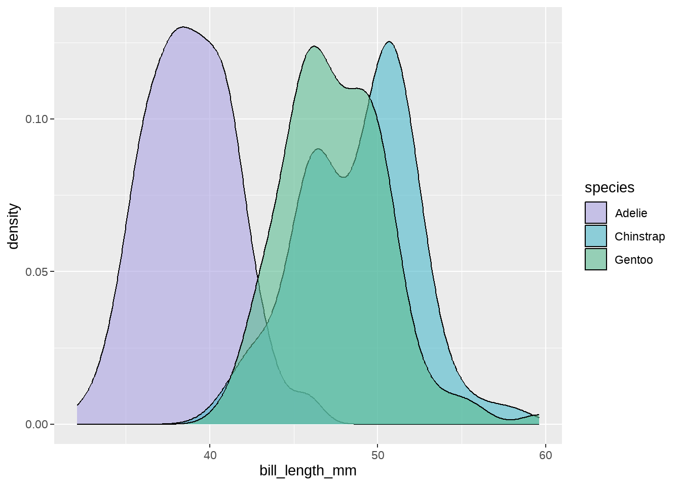
penguins %>%
   ggplot(aes(bill_length_mm, fill = species)) +
   geom_density(alpha = 0.6) +
   scale_fill_discrete_qualitative(palette = "cold", nmax = 4, order = 2:4)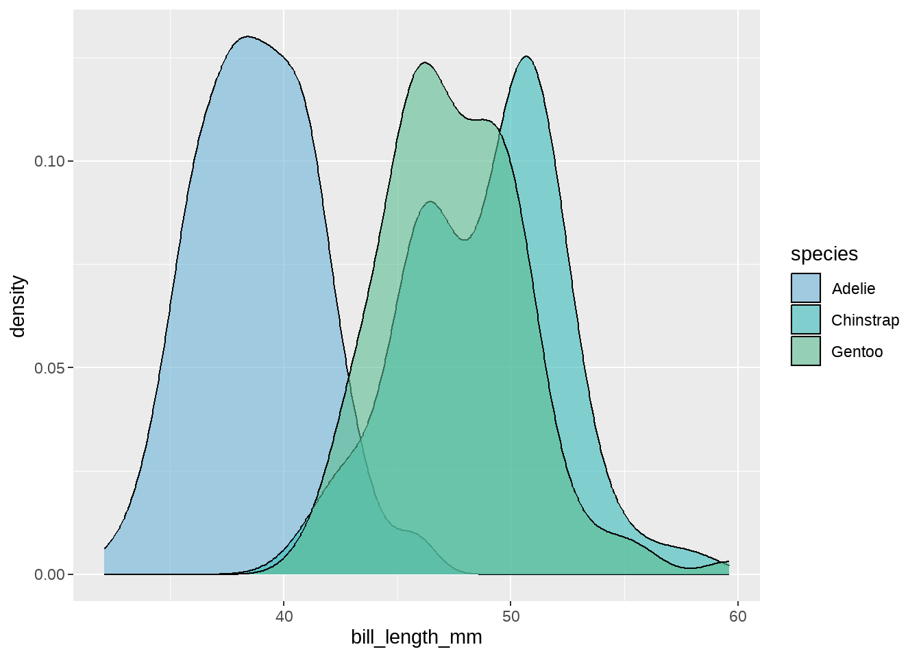
sequential_hcl(palette = "Purples 3", n = 6) %>%
  swatchplot()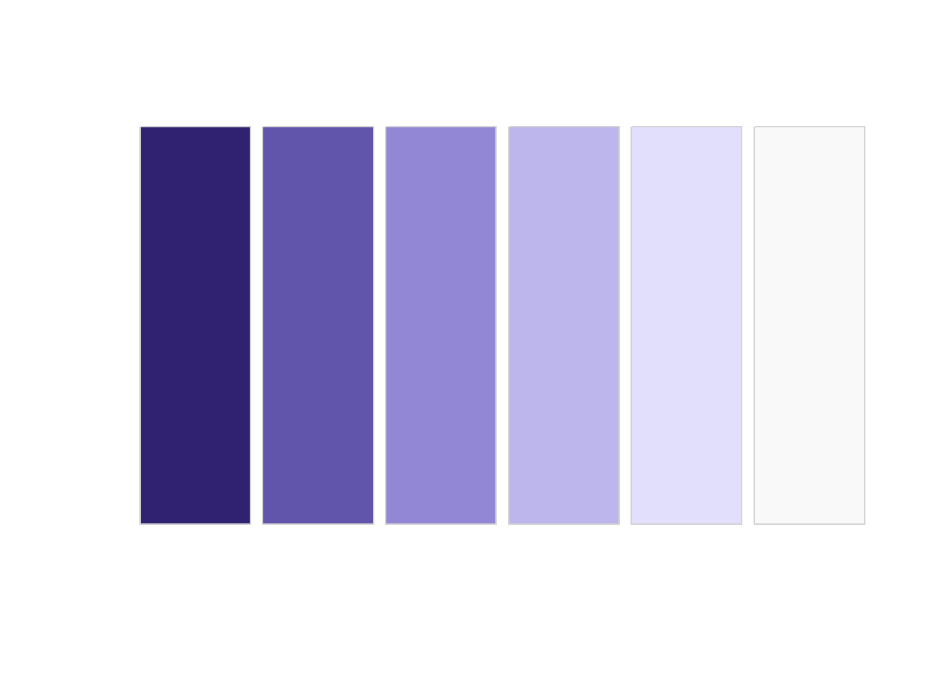
penguins %>%
   ggplot(aes(bill_length_mm, fill = species)) +
   geom_density(alpha = 0.6) +
   scale_fill_discrete_sequential(palette = "Purples 3",
                                  nmax = 6,
                                  rev = FALSE,
                                  order = 3:5)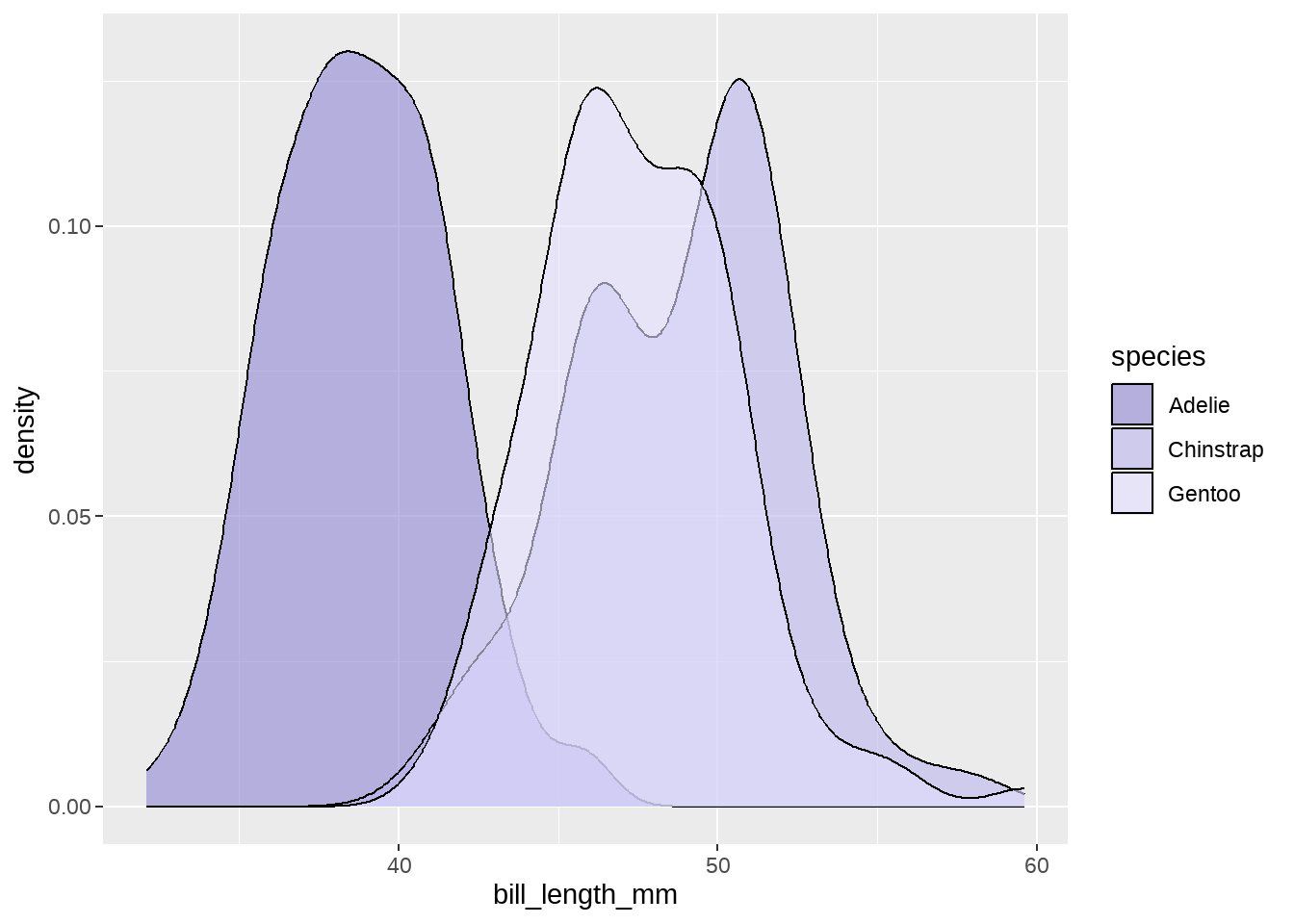
29.4 使用案例2
temps_months <- read_csv("./demo_data/tempnormals.csv") %>%
  group_by(location, month_name) %>%
  summarize(mean = mean(temperature)) %>%
  mutate(
    month = factor(
      month_name,
      levels = c("Jan", "Feb", "Mar", "Apr", "May", "Jun", "Jul", "Aug", "Sep", "Oct", "Nov", "Dec")
    ),
    location = factor(
      location, levels = c("Death Valley", "Houston", "San Diego", "Chicago")
    )
  ) %>%
  select(-month_name)

temps_months
## # A tibble: 48 × 3
## # Groups: location [4]
## location mean month
## <fct> <dbl> <fct>
## 1 Chicago 50.4 Apr
## 2 Chicago 74.1 Aug
## 3 Chicago 29 Dec
## 4 Chicago 28.9 Feb
## 5 Chicago 24.8 Jan
## 6 Chicago 75.8 Jul
## 7 Chicago 71.0 Jun
## 8 Chicago 38.8 Mar
## 9 Chicago 60.9 May
## 10 Chicago 41.6 Nov
## # ℹ 38 more rows
temps_months %>%
  ggplot(aes(x = month, y = location, fill = mean)) +
  geom_tile(width = 0.95, height = 0.95) +
  coord_fixed(expand = FALSE) +
  theme_classic()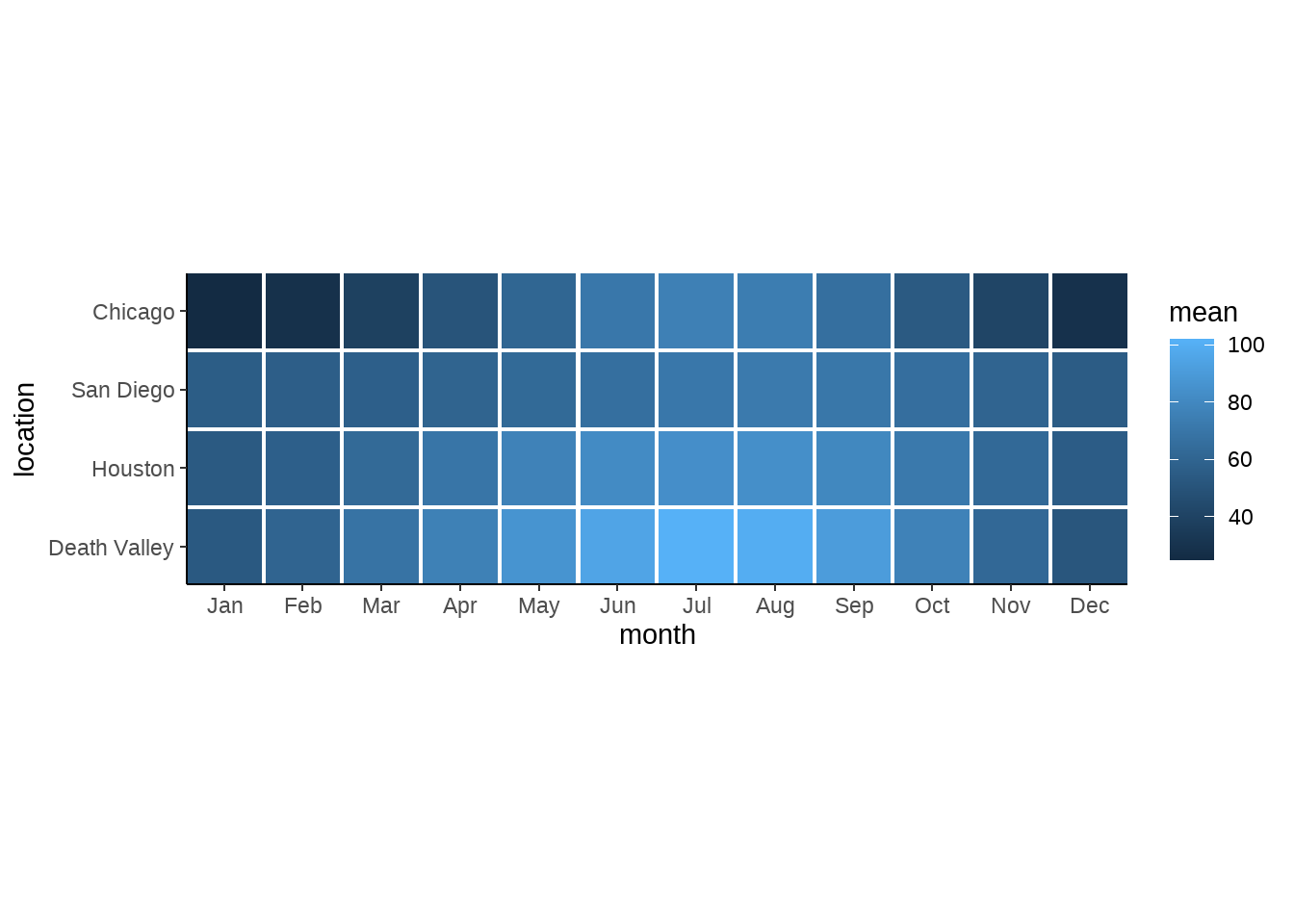
temps_months %>%
  ggplot(aes(x = month, y = location, fill = mean)) +
  geom_tile(width = 0.95, height = 0.95) +
  coord_fixed(expand = FALSE) +
  theme_classic() +
  scale_fill_gradient()
temps_months %>%
  ggplot(aes(x = month, y = location, fill = mean)) +
  geom_tile(width = 0.95, height = 0.95) +
  coord_fixed(expand = FALSE) +
  theme_classic() +
  scale_fill_viridis_c()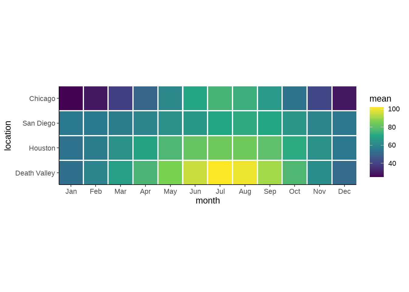
temps_months %>%
  ggplot(aes(x = month, y = location, fill = mean)) +
  geom_tile(width = 0.95, height = 0.95) +
  coord_fixed(expand = FALSE) +
  theme_classic() +
  scale_fill_viridis_c(option = "B", begin = 0.15)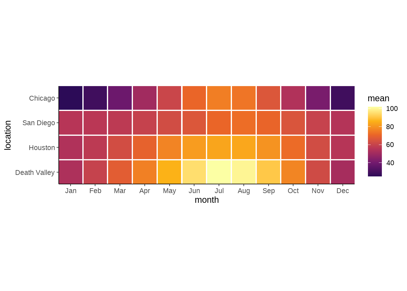
temps_months %>%
  ggplot(aes(x = month, y = location, fill = mean)) +
  geom_tile(width = 0.95, height = 0.95) +
  coord_fixed(expand = FALSE) +
  theme_classic() +
  scale_fill_continuous_sequential(palette = "YlGnBu", rev = FALSE)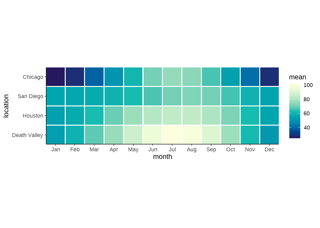
temps_months %>%
  ggplot(aes(x = month, y = location, fill = mean)) +
  geom_tile(width = 0.95, height = 0.95) +
  coord_fixed(expand = FALSE) +
  theme_classic() +
  scale_fill_continuous_sequential(palette = "Viridis", rev = FALSE)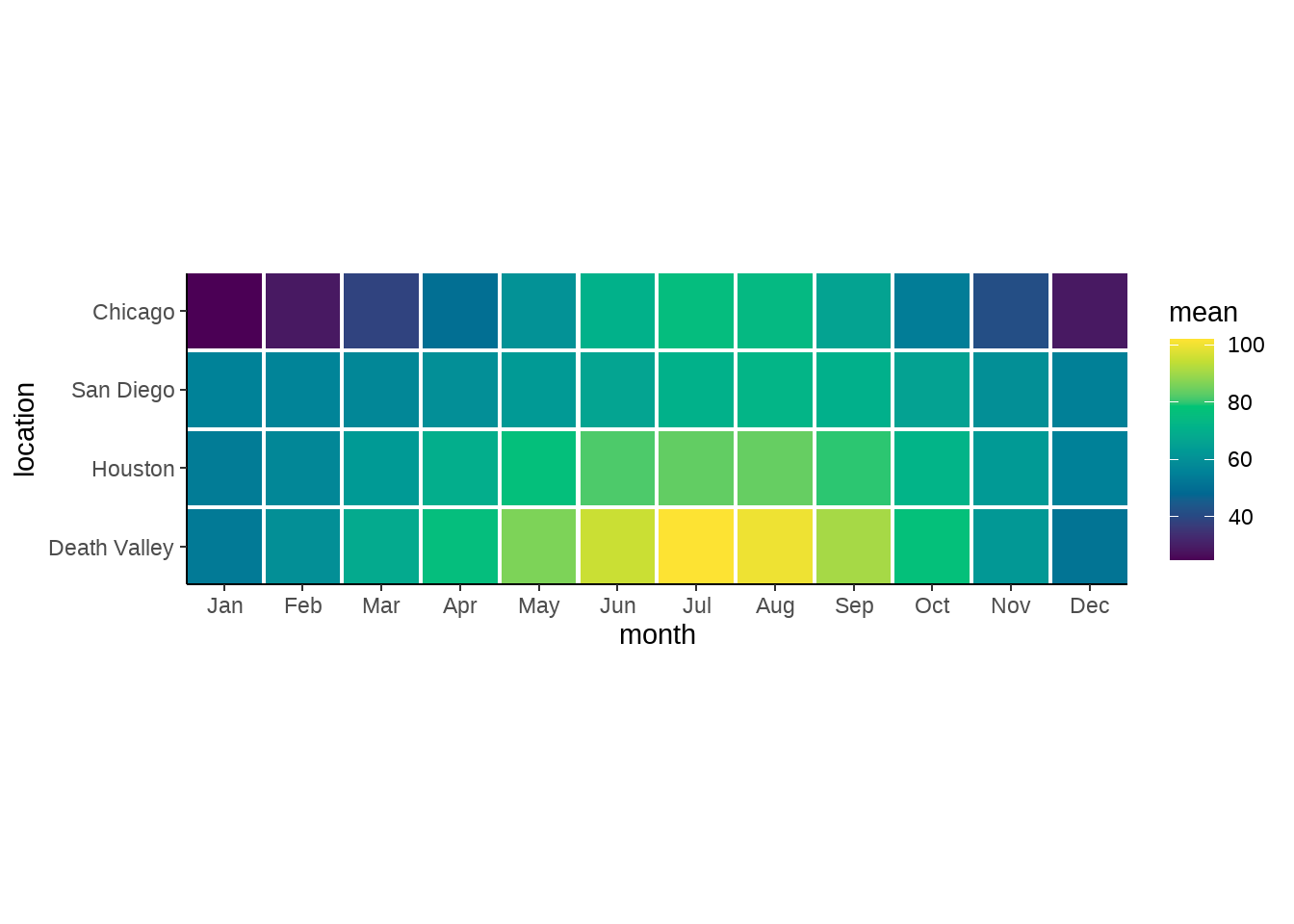
temps_months %>%
  ggplot( aes(x = month, y = location, fill = mean)) +
  geom_tile(width = 0.95, height = 0.95) +
  coord_fixed(expand = FALSE) +
  theme_classic() +
  scale_fill_continuous_sequential(palette = "Inferno", begin = 0.15, rev = FALSE)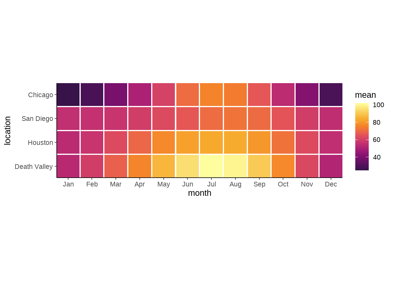
temps_months %>%
  ggplot(aes(x = month, y = location, fill = mean)) +
  geom_tile(width = 0.95, height = 0.95) +
  coord_fixed(expand = FALSE) +
  theme_classic() +
  scale_fill_continuous_sequential(palette = "Plasma", begin = 0.35, rev = FALSE)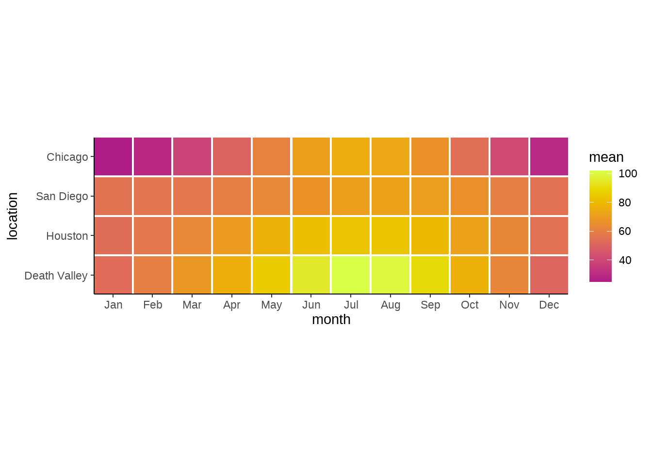
29.5 配色
这里有个小小的提示:
- 尽可能避免使用
"red","green","blue","cyan","magenta","yellow"颜色 - 使用相对柔和的颜色
"firebrick","springgreen4","blue3","turquoise3","darkorchid2","gold2",会让人觉得舒服
可以对比下
colorspace::swatchplot(c("red", "green", "blue", "cyan", "magenta", "yellow"))
colorspace::swatchplot(c("firebrick", "springgreen4", "blue3", "turquoise3", "darkorchid2", "gold2"))