第 18 章 因子型变量
本章介绍R语言中的因子类型数据。因子型变量常用于数据处理和可视化中,尤其在希望不以字母顺序排序的时候,因子就格外有用。
18.1 什么是因子
因子是把数据进行分类并标记为不同层级(level,有时候也翻译成因子水平, 我个人觉得翻译为层级,更接近它的特性,因此,我都会用层级来描述)的数据对象,他们可以存储字符串和整数。因子类型有三个属性:
- 存储类别的数据类型
- 离散变量
- 因子的层级是有限的,只能取因子层级中的值或缺失(NA)
18.2 创建因子
## [1] low    high   medium medium low    high   high
## Levels: high low medium因子层级会自动按照字符串的字母顺序排序,比如high low medium。也可以指定顺序,
## [1] low    high   medium medium low    high   high
## Levels: low high medium
不属于因子层级中的值, 比如这里因子层只有c("low", "high"),那么income中的”medium”会被当作缺省值NA
## [1] low  high <NA> <NA> low  high high
## Levels: low high
相比较字符串而言,因子类型更容易处理,因此很多函数会自动的将字符串转换为因子来处理,但事实上,这也会造成,不想当做因子的却又当做了因子的情形,最典型的是在R 4.0之前,data.frame()中stringsAsFactors选项,默认将字符串类型转换为因子类型,但这个默认也带来一些不方便,因此在R 4.0之后取消了这个默认。在tidyverse集合里,有专门处理因子的宏包forcats,因此,本章将围绕forcats宏包讲解如何处理因子类型变量,更多内容可以参考这里。
18.3 调整因子顺序
前面看到因子层级是按照字母顺序排序
x <- factor(income)
x
## [1] low high medium medium low high high
## Levels: high low medium也可以指定顺序
x %>% fct_relevel( c("high", "medium", "low"))## [1] low high medium medium low high high
## Levels: high medium low或者让”medium” 移动到最前面
x %>% fct_relevel( c("medium"))## [1] low high medium medium low high high
## Levels: medium high low或者让”medium” 移动到最后面
x %>% fct_relevel("medium", after = Inf)## [1] low high medium medium low high high
## Levels: high low medium可以按照字符串第一次出现的次序
x %>% fct_inorder()## [1] low high medium medium low high high
## Levels: low high medium按照其他变量的中位数的升序排序
x %>% fct_reorder(c(1:7), .fun = median) ## [1] low high medium medium low high high
## Levels: low medium high18.4 应用
调整因子层级有什么用呢?
这个功能在ggplot可视化中调整分类变量的顺序非常方便。这里为了方便演示,我们假定有数据框
## # A tibble: 6 × 2
## x y
## <chr> <dbl>
## 1 a 2
## 2 a 2
## 3 b 1
## 4 b 5
## 5 c 0
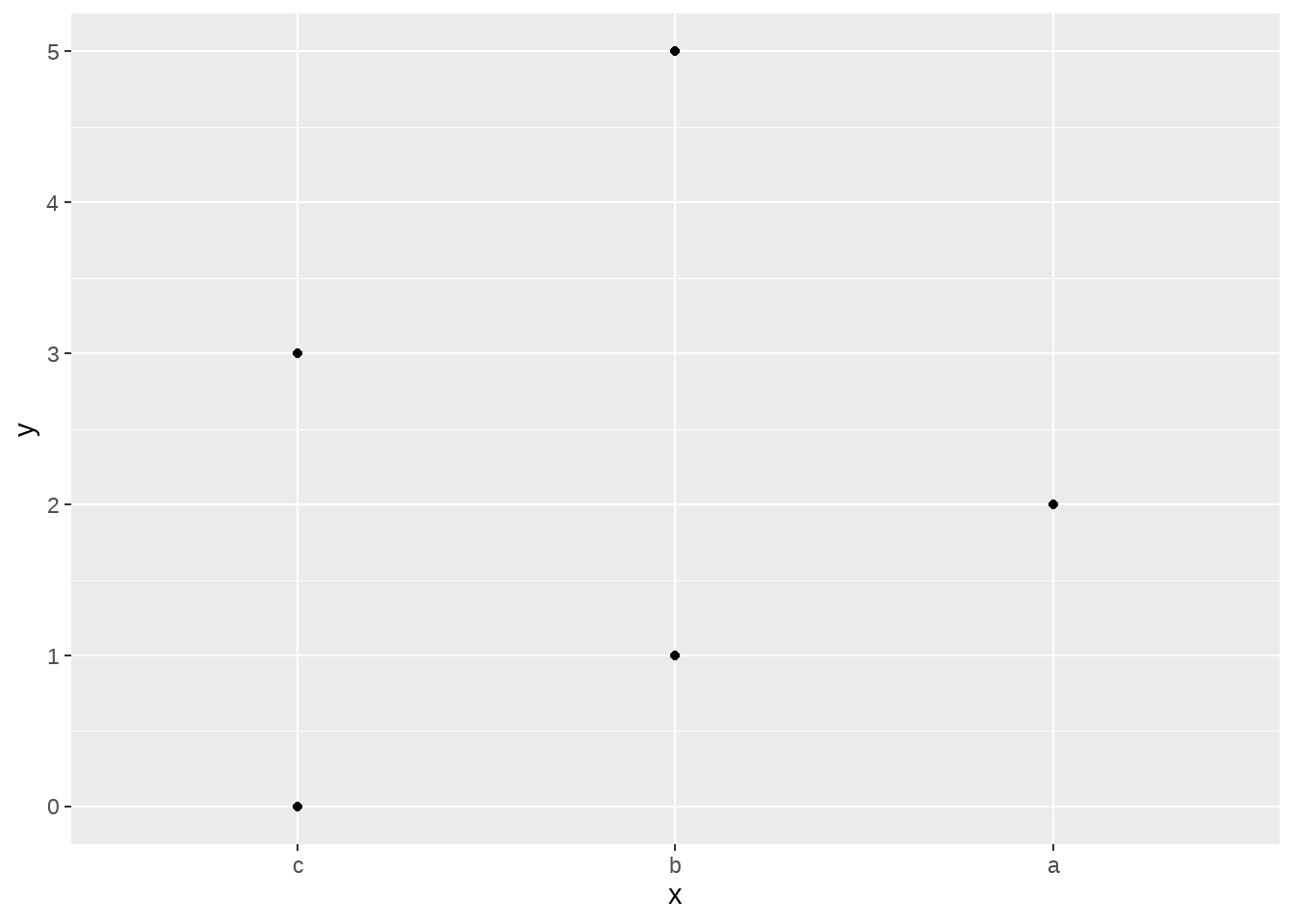
## 6 c 3先画个散点图看看吧
d %>%
  ggplot(aes(x = x, y = y)) +
  geom_point()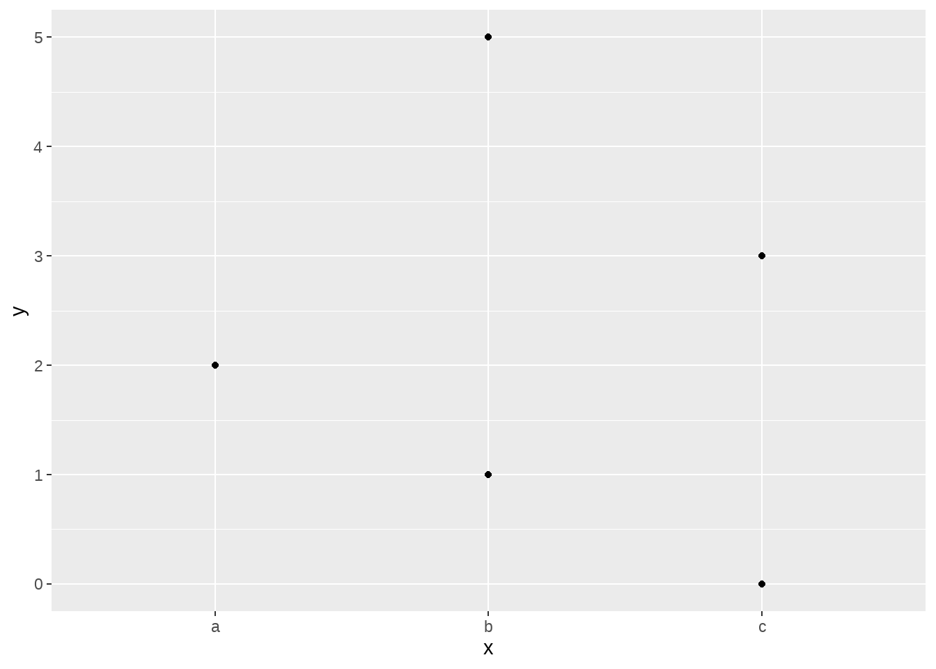
我们看到,横坐标上是a-b-c的顺序。
18.4.1 fct_reorder()
fct_reorder()可以让x的顺序按照x中每个分类变量对应y值的中位数升序排序,具体为
- a对应的y值
c(2, 2)中位数是median(c(2, 2)) = 2 - b对应的y值
c(1, 5)中位数是median(c(1, 5)) = 3 - c对应的y值
c(0, 3)中位数是median(c(0, 3)) = 1.5
因此,x的因子层级的顺序调整为c-a-b
d %>%
  ggplot(aes(x = fct_reorder(x, y, .fun = median), y = y)) +
  geom_point()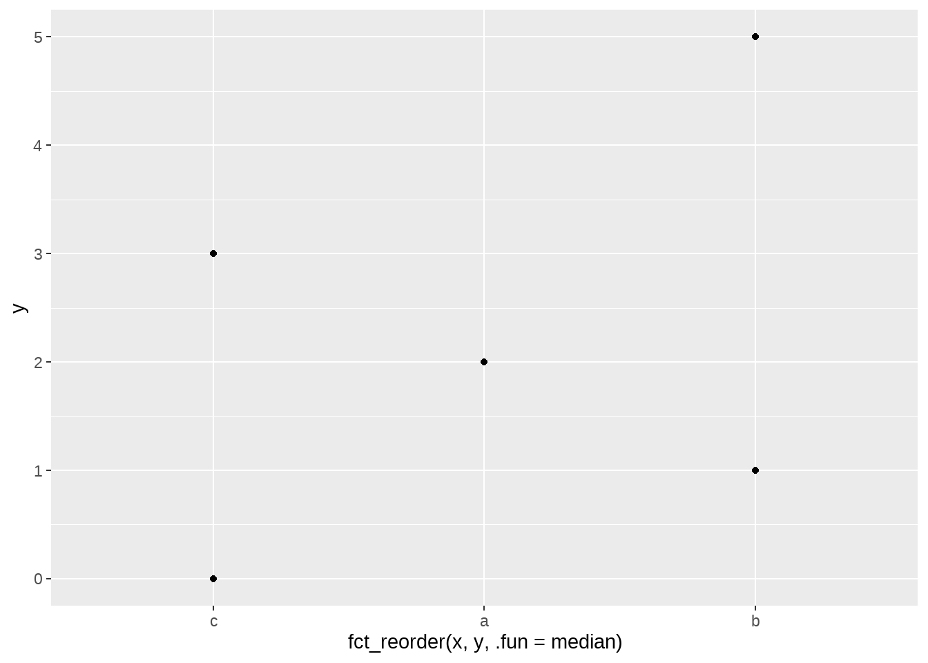
当然,我们可以加一个参数.desc = TRUE让因子层级变为降序排列b-a-c
d %>%
  ggplot(aes(x = fct_reorder(x, y, .fun = median, .desc = TRUE), y = y)) +
  geom_point()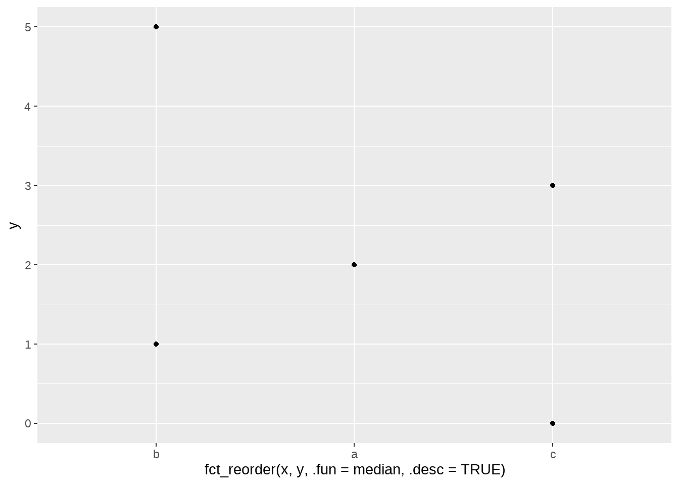
但这样会造成x坐标标签一大串,因此建议可以写mutate()函数里
d %>%
  mutate(x = fct_reorder(x, y, .fun = median, .desc = TRUE)) %>%
  ggplot(aes(x = x, y = y)) +
  geom_point()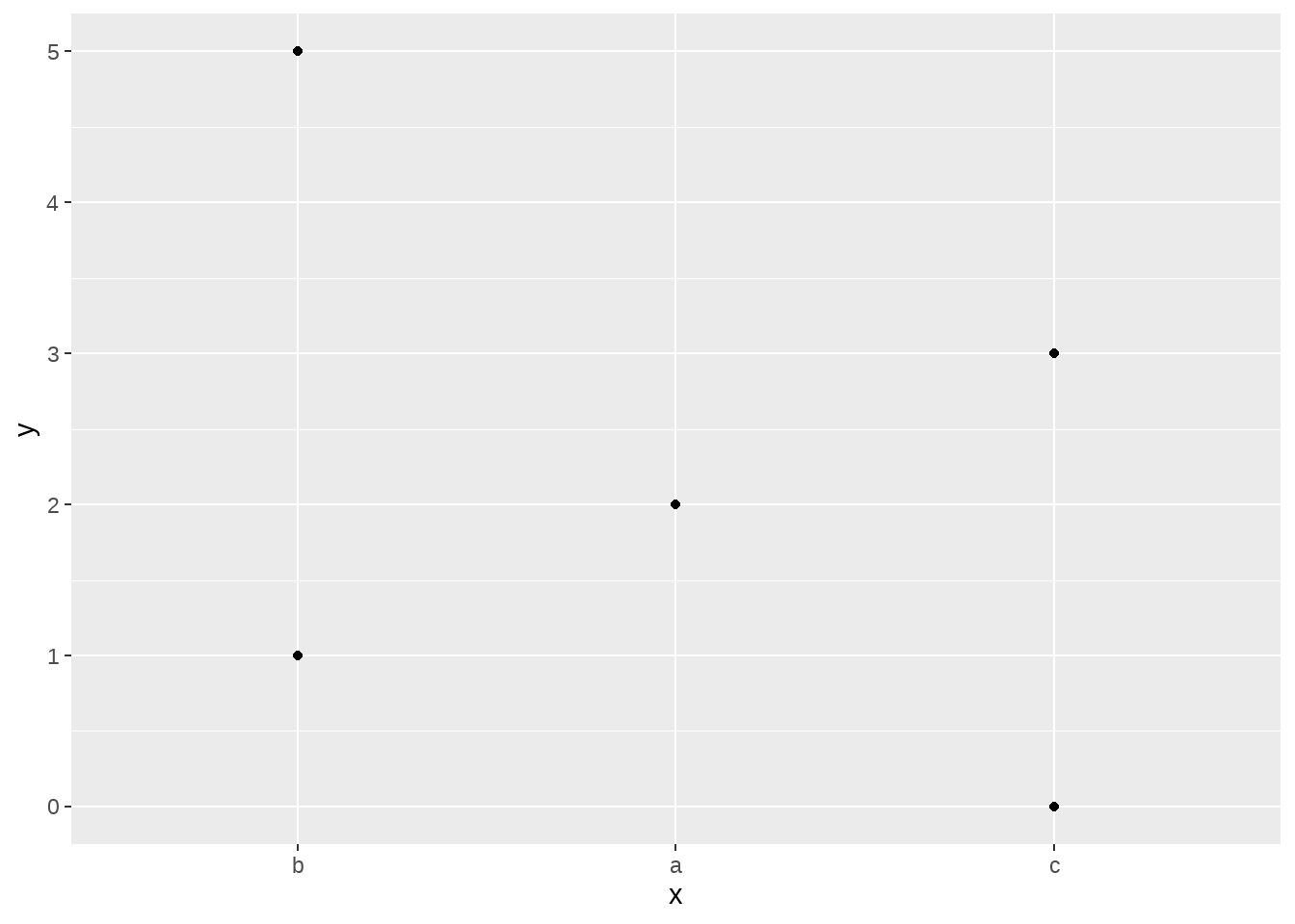
我们还可以按照y值中最小值的大小降序排列
d %>%
  mutate(x = fct_reorder(x, y, .fun = min, .desc = TRUE)) %>%
  ggplot(aes(x = x, y = y)) +
  geom_point()
18.4.3 fct_relevel()
d %>%
  mutate(
    x = fct_relevel(x, c("c", "a", "b"))
  ) %>%

  ggplot(aes(x = x, y = y)) +
  geom_point()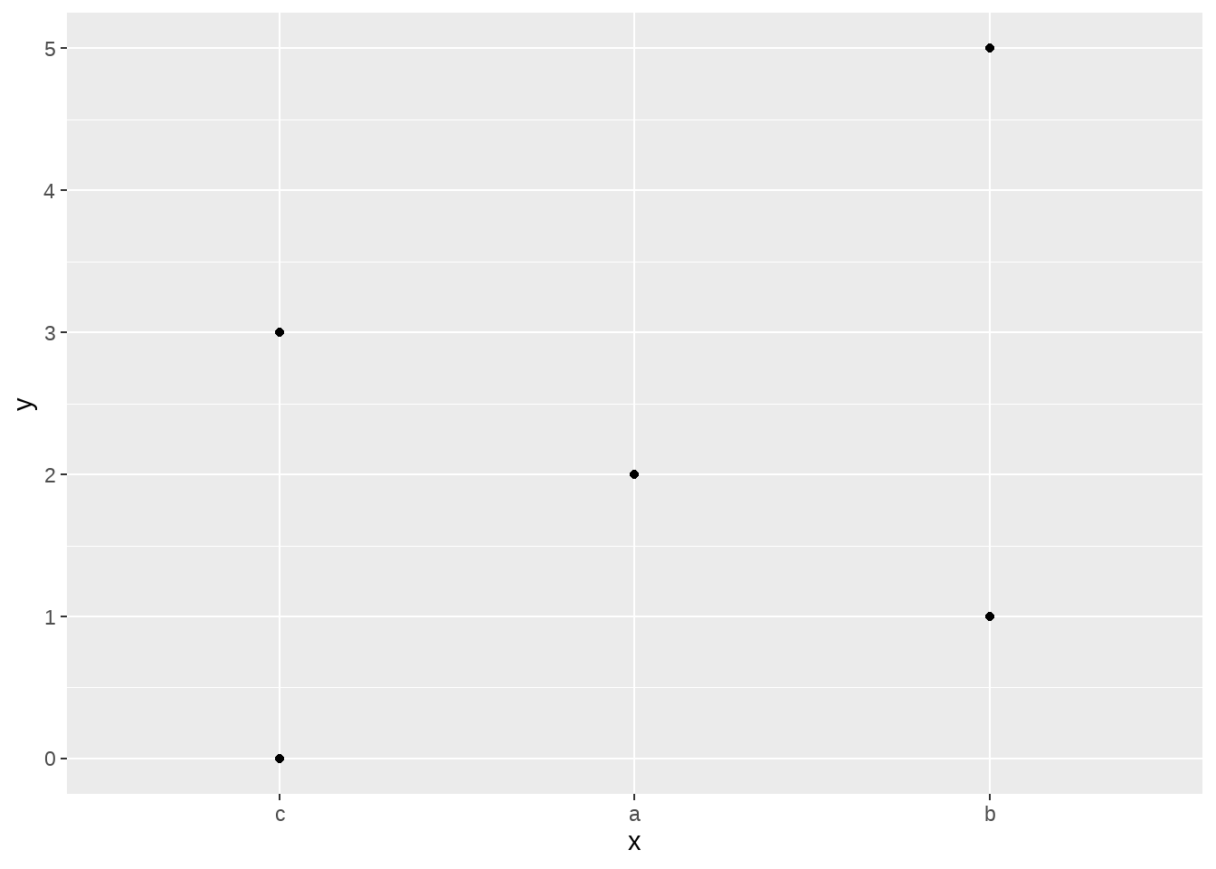
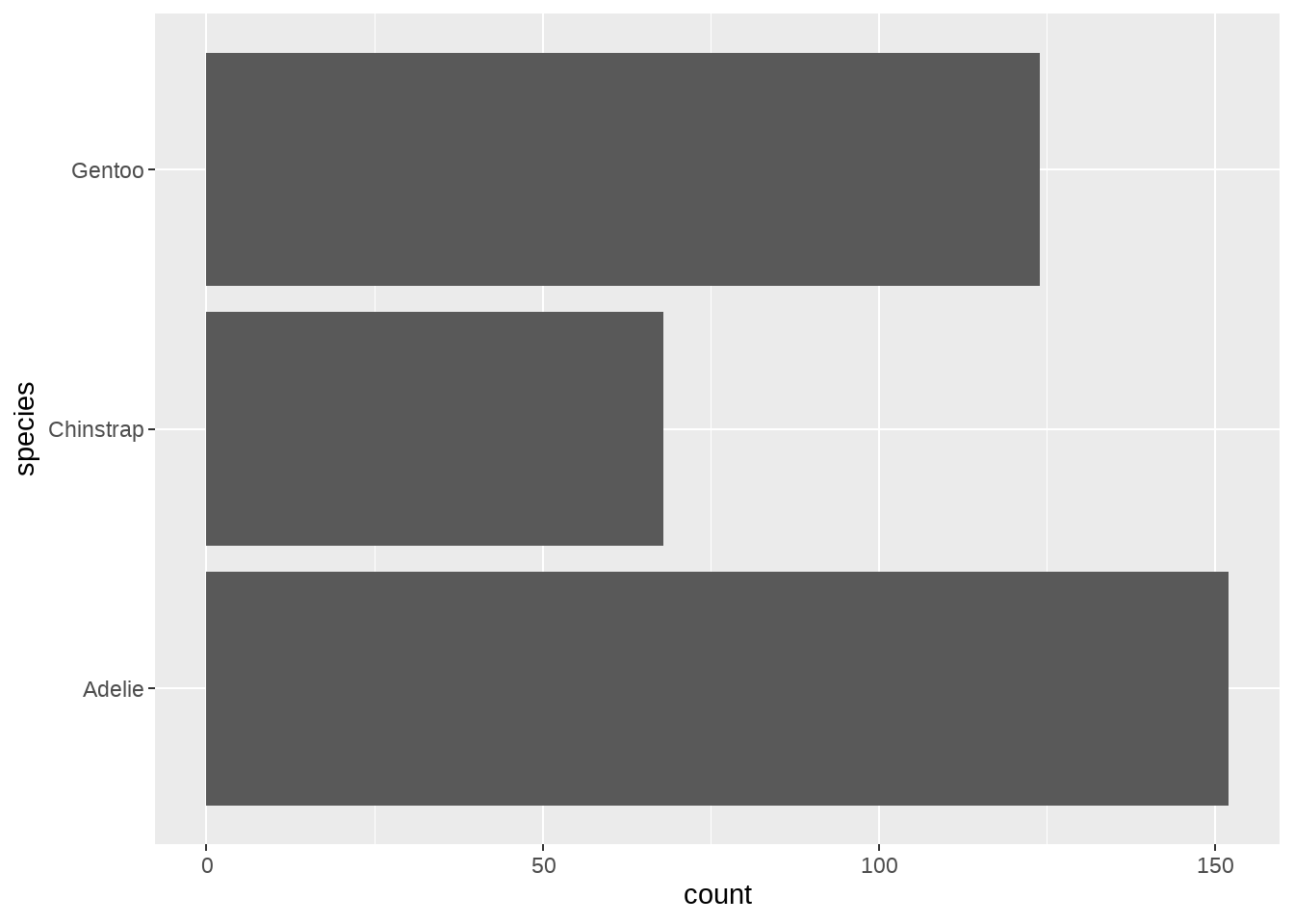
18.5 可视化中应用
可能没说明白,那就看企鹅柱状图吧
penguins %>%
  count(species) %>%
  pull(species)

penguins %>%
  count(species) %>%
  mutate(species = fct_relevel(species, "Chinstrap", "Gentoo", "Adelie")) %>%
  pull(species)
# Move "Chinstrap" in front, rest alphabetic
ggplot(penguins, aes(y = fct_relevel(species, "Chinstrap"))) +
  geom_bar()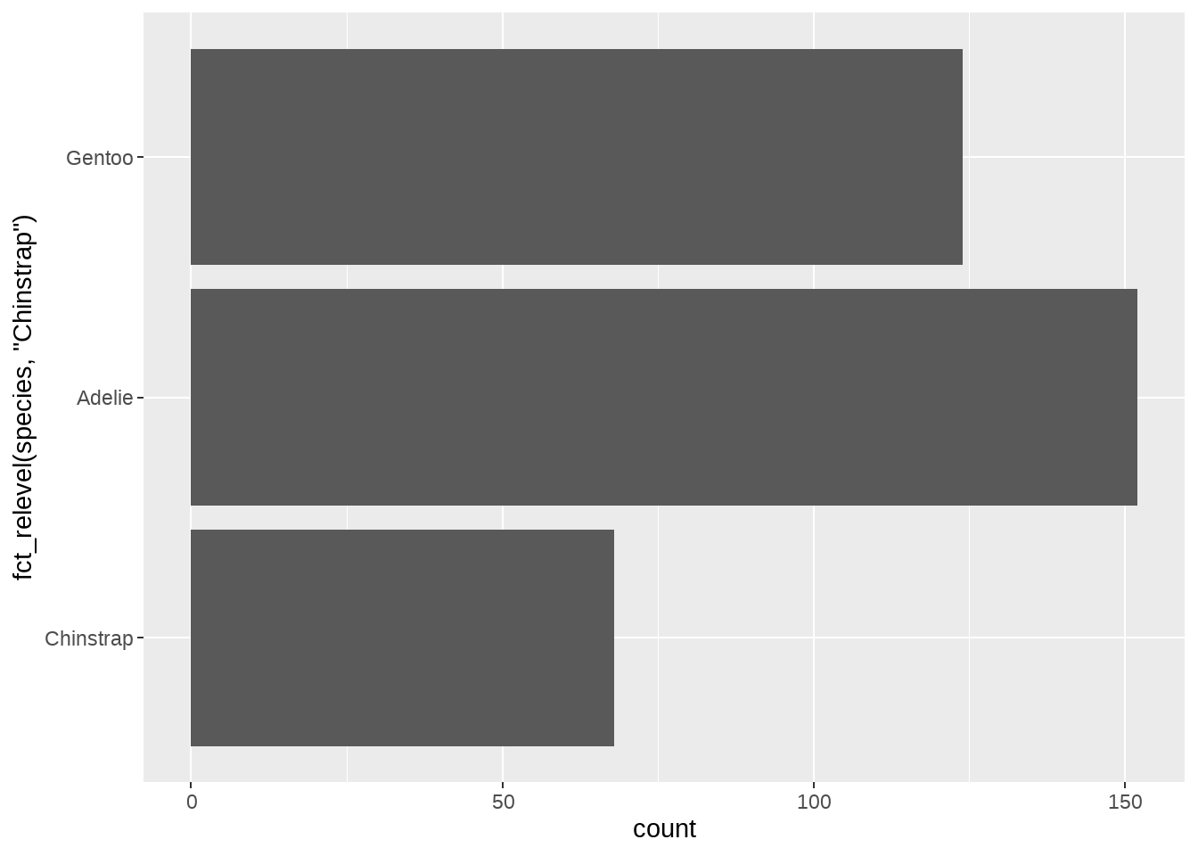
# Use order "Chinstrap", "Gentoo", "Adelie"
ggplot(penguins, aes(y = fct_relevel(species, "Chinstrap", "Gentoo", "Adelie"))) +
  geom_bar()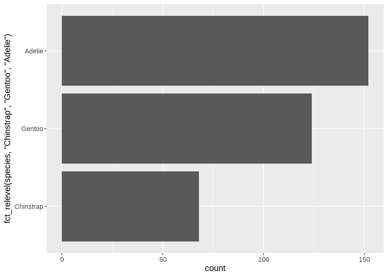
penguins %>%
  mutate(species = fct_relevel(species, "Chinstrap", "Gentoo", "Adelie")) %>%
  ggplot(aes(y = species)) +
  geom_bar()
ggplot(penguins, aes(y = fct_relevel(species, "Adelie", after = Inf))) +
  geom_bar()
# Use the order defined by the number of penguins of different species
# The order is descending, from most frequent to least frequent

penguins %>%
  mutate(species = fct_infreq(species)) %>%
  ggplot(aes(y = species)) +
  geom_bar()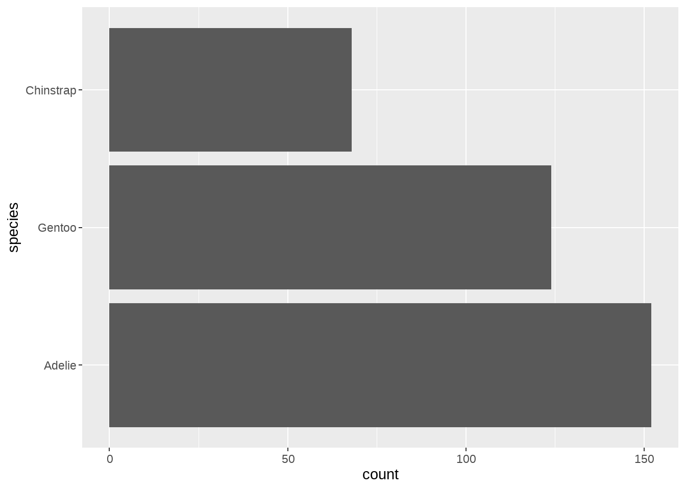
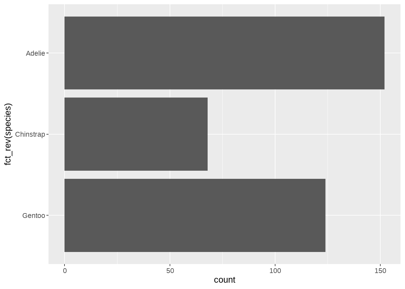
penguins %>%
  mutate(species = fct_rev(fct_infreq(species))) %>%
  ggplot(aes(y = species)) +
  geom_bar()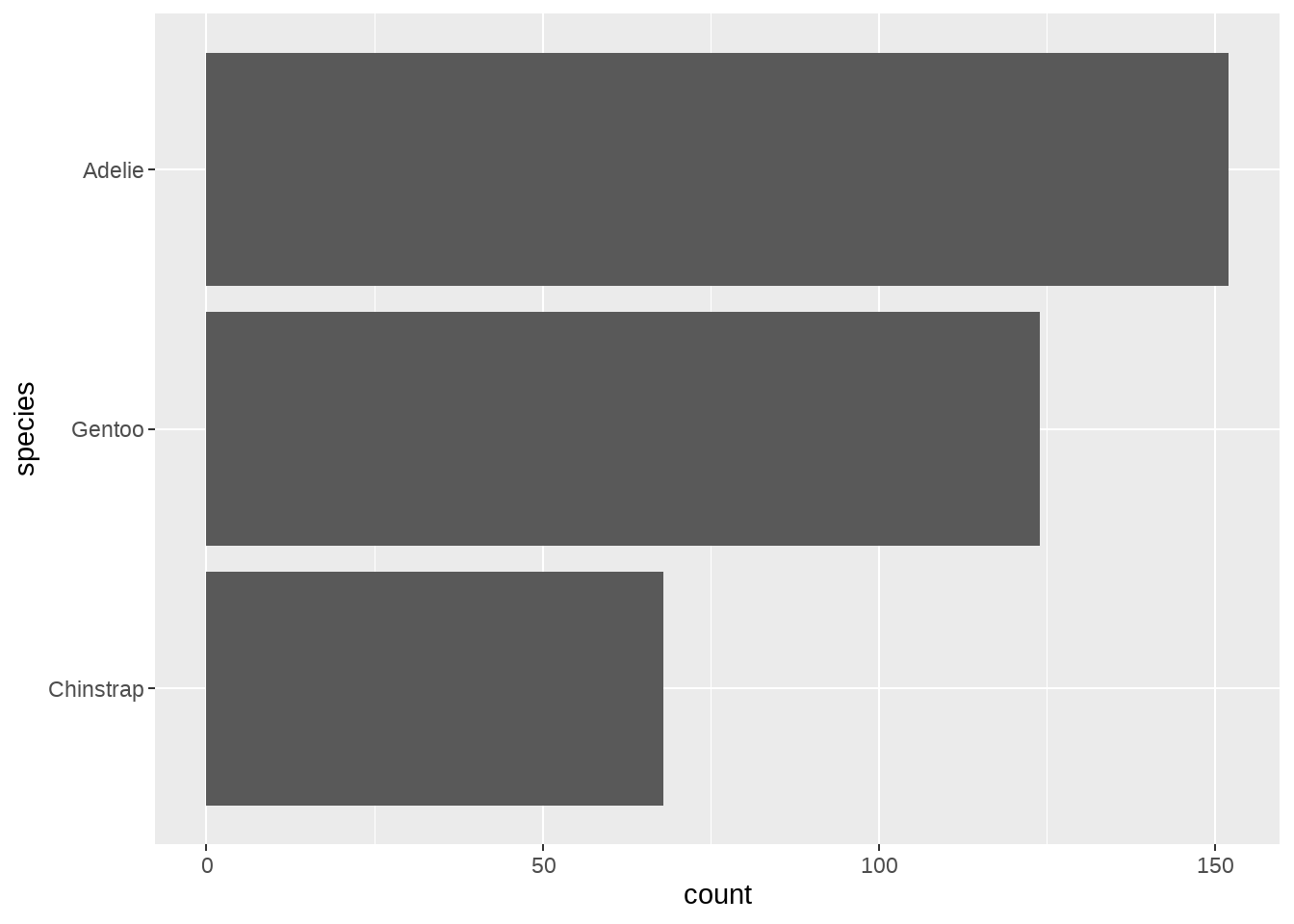
# Reorder based on numeric values
penguins %>%
  count(species) %>%
  mutate(species = fct_reorder(species, n)) %>%
  ggplot(aes(n, species)) +
  geom_col()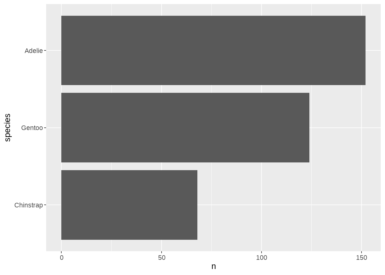
18.6 作业
- 画出的2007年美洲人口寿命的柱状图,要求从高到低排序
## # A tibble: 25 × 6
##    country            continent  year lifeExp       pop gdpPercap
##    <fct>              <fct>     <int>   <dbl>     <int>     <dbl>
##  1 Argentina          Americas   2007    75.3  40301927    12779.
##  2 Bolivia            Americas   2007    65.6   9119152     3822.
##  3 Brazil             Americas   2007    72.4 190010647     9066.
##  4 Canada             Americas   2007    80.7  33390141    36319.
##  5 Chile              Americas   2007    78.6  16284741    13172.
##  6 Colombia           Americas   2007    72.9  44227550     7007.
##  7 Costa Rica         Americas   2007    78.8   4133884     9645.
##  8 Cuba               Americas   2007    78.3  11416987     8948.
##  9 Dominican Republic Americas   2007    72.2   9319622     6025.
## 10 Ecuador            Americas   2007    75.0  13755680     6873.
## # ℹ 15 more rows- 这是四个国家人口寿命的变化图
gapminder %>%
  filter(country %in% c("Norway", "Portugal", "Spain", "Austria")) %>%
  ggplot(aes(year, lifeExp)) + geom_line() +
  facet_wrap(vars(country), nrow = 1)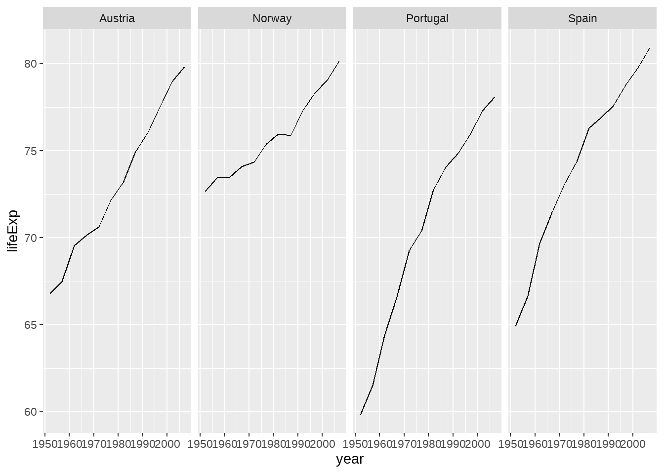
要求给四个分面排序,按每个国家寿命的中位数
要求给四个分面排序,按每个国家寿命差(最大值减去最小值)