第 51 章 线性回归
线性模型是数据分析中最常用的一种分析方法。最基础的往往最深刻。
51.1 从一个案例开始
这是一份1994年收集1379个对象关于收入、身高、教育水平等信息的数据集。数据可以在这里下载。
首先,我们下载后导入数据
## # A tibble: 6 × 6
##     earn height sex    race     ed   age
##    <dbl>  <dbl> <chr>  <chr> <dbl> <dbl>
## 1 79571.   73.9 male   white    16    49
## 2 96397.   66.2 female white    16    62
## 3 48711.   63.8 female white    16    33
## 4 80478.   63.2 female other    16    95
## 5 82089.   63.1 female white    17    43
## 6 15313.   64.5 female white    15    30
51.1.1 缺失值检查
一般情况下,拿到一份数据,首先要了解数据,知道每个变量的含义,
## [1] "earn" "height" "sex" "race" "ed" "age"同时检查数据是否有缺失值,这点很重要。在R中 NA(not available,不可用)表示缺失值, 比如可以这样检查是否有缺失值。
wages %>%
  summarise(
    earn_na   = sum(is.na(earn)),
    height_na = sum(is.na(height)),
    sex_na    = sum(is.na(sex)),
    race_na   = sum(is.na(race)),
    ed_na     = sum(is.na(ed)),
    age_na    = sum(is.na(age))
  )
## # A tibble: 1 × 6
## earn_na height_na sex_na race_na ed_na age_na
## <int> <int> <int> <int> <int> <int>
## 1 0 0 0 0 0 0程序员都是偷懒的,所以也可以写的简便一点。大家在学习的过程中,也会慢慢的发现tidyverse的函数很贴心,很周到。
wages %>%
  summarise_all(
    ~ sum(is.na(.))
  )
## # A tibble: 1 × 6
## earn height sex race ed age
## <int> <int> <int> <int> <int> <int>
## 1 0 0 0 0 0 0当然,也可以用purrr::map()的方法。这部分我会在后面的章节中逐步介绍。
## # A tibble: 1 × 6
##    earn height   sex  race    ed   age
##   <int>  <int> <int> <int> <int> <int>
## 1 0 0 0 0 0 051.1.2 变量简单统计
然后探索下每个变量的分布。比如调研数据中男女的数量分别是多少?
## # A tibble: 2 × 2
##   sex        n
##   <chr>  <int>
## 1 female   859
## 2 male     520
男女这两组的身高均值分别是多少?收入的均值分别是多少?
wages %>%
  group_by(sex) %>%
  summarise(
    n = n(),
    mean_height = mean(height),
    mean_earn = mean(earn)
  )
## # A tibble: 2 × 4
## sex n mean_height mean_earn
## <chr> <int> <dbl> <dbl>
## 1 female 859 64.5 24246.
## 2 male 520 70.0 45993.也有可以用可视化的方法,呈现男女收入的分布情况
wages %>%
  ggplot(aes(x = earn, color = sex)) +
  geom_density()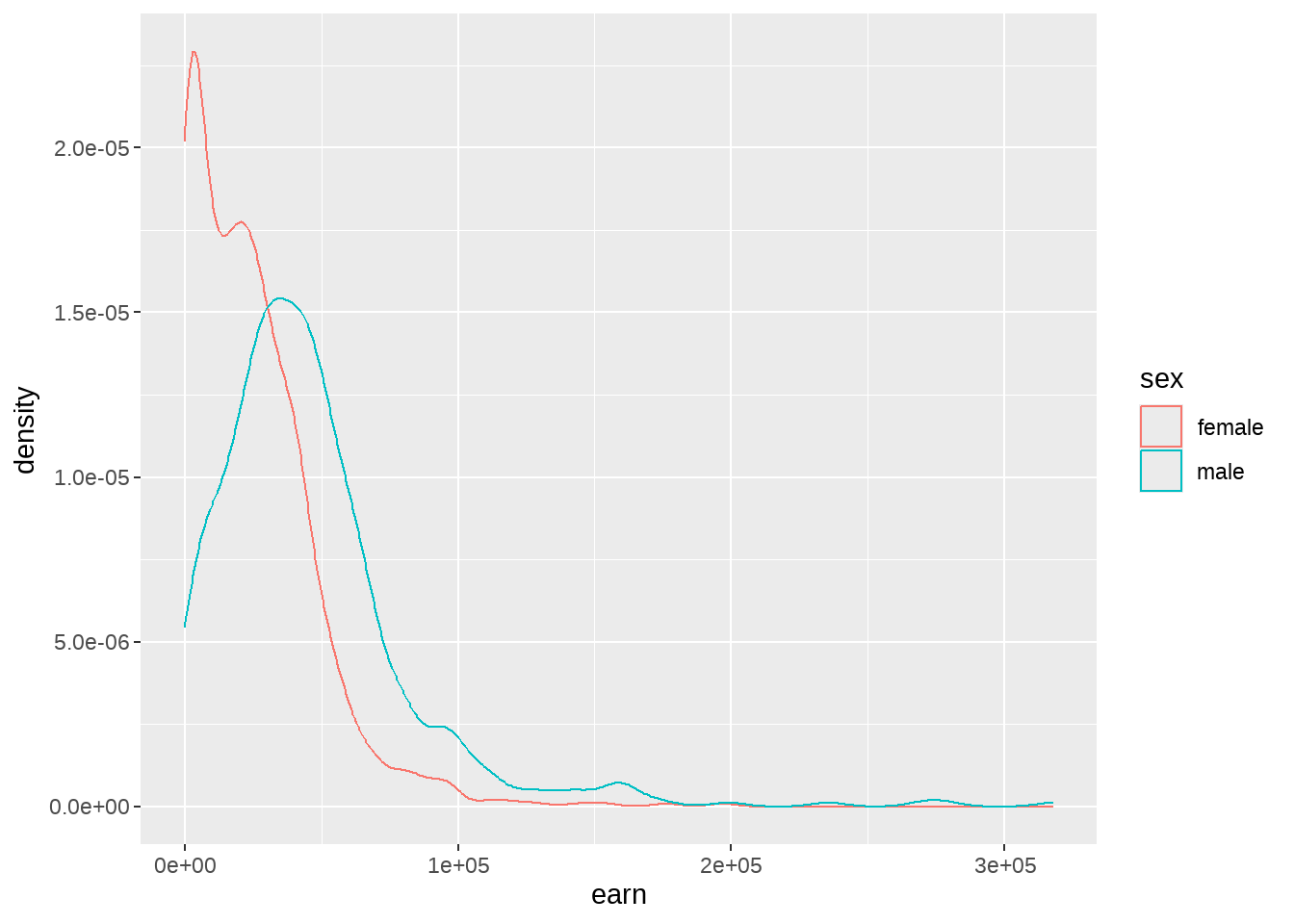
大家可以自行探索其他变量的情况。现在提出几个问题,希望大家带着这些问题去探索:
长的越高的人挣钱越多?
是否男性就比女性挣的多?
影响收入最大的变量是哪个?
怎么判定我们建立的模型是不是很好?
51.2 线性回归模型
长的越高的人挣钱越多?
要回答这个问题,我们先介绍线性模型。顾名思义,就是认为\(x\)和\(y\)之间有线性关系,数学上可以写为
\[ \begin{aligned} y &= \alpha + \beta x + \epsilon \\ \epsilon &\in \text{Normal}(\mu, \sigma) \end{aligned} \]
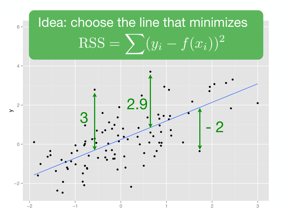
\(\epsilon\) 代表误差项,它与\(x\) 无关,且服从正态分布。 建立线性模型,就是要估计这里的系数\(\hat\alpha\)和\(\hat\beta\),即截距项和斜率项。常用的方法是最小二乘法(ordinary least squares (OLS) regression): 就是我们估算的\(\hat\alpha\)和\(\hat\beta\), 要使得残差的平方和最小,即\(\sum_i(y_i - \hat y_i)^2\)或者叫\(\sum_i \epsilon_i^2\)最小。
当然,数据量很大,手算是不现实的,我们借助R语言代码吧
51.3 使用lm() 函数
用R语言代码(建议大家先?lm看看帮助文档),
lm参数很多, 但很多我们都用不上,所以我们只关注其中重要的两个参数
lm(formula = y ~ x, data)lm(y ~ x, data) 是最常用的线性模型函数(lm是linear model的缩写)。参数解释说明
-
formula:指定回归模型的公式,对于简单的线性回归模型
y ~ x. -
~
符号:代表“预测”,可以读做“y由x预测”。有些学科不同的表述,比如下面都是可以的
-
response ~ explanatory
-
dependent ~ independent -
outcome ~ predictors
-
- data:代表数据框,数据框包含了响应变量和独立变量
在运行lm()之前,先画出身高和收入的散点图(记在我们想干什么,寻找身高和收入的关系)
wages %>%
  ggplot(aes(x = height, y = earn)) +
  geom_point()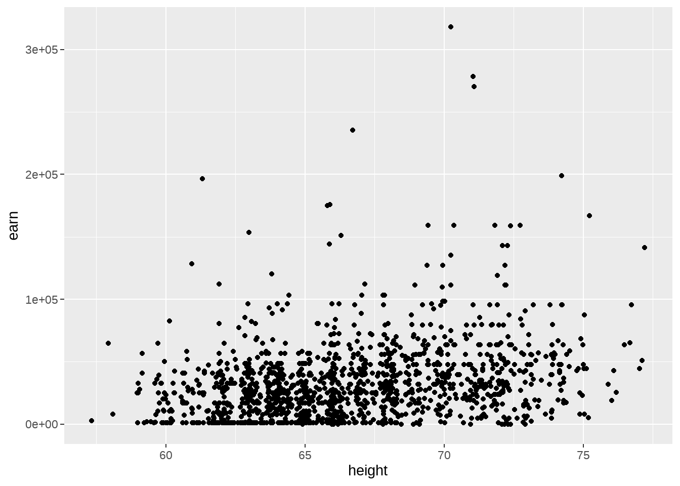
等不及了,就运行代码吧
mod1 <- lm(
  formula = earn ~ height,
  data = wages
)这里我们将earn作为响应变量,height为预测变量。lm()返回赋值给mod1. mod1现在是个什么东东呢? mod1是一个叫lm object或者叫类的东西,
names(mod1)## [1] "coefficients" "residuals" "effects" "rank"
## [5] "fitted.values" "assign" "qr" "df.residual"
## [9] "xlevels" "call" "terms" "model"我们打印看看,会发生什么
print(mod1)##
## Call:
## lm(formula = earn ~ height, data = wages)
##
## Coefficients:
## (Intercept) height
## -126523 2387这里有两部分信息。首先第一部分是我们建立的模型;第二部分是R给出了截距(\(\alpha = -126532\))和斜率(\(\beta = 2387\)). 也就是说我们建立的线性回归模型是 \[ \hat y = -126532 + 2387 \; x \]
查看详细信息
summary(mod1)##
## Call:
## lm(formula = earn ~ height, data = wages)
##
## Residuals:
## Min 1Q Median 3Q Max
## -47903 -19744 -5184 11642 276796
##
## Coefficients:
## Estimate Std. Error t value Pr(>|t|)
## (Intercept) -126523 14076 -8.989 <2e-16 ***
## height 2387 211 11.312 <2e-16 ***
## ---
## Signif. codes: 0 '***' 0.001 '**' 0.01 '*' 0.05 '.' 0.1 ' ' 1
##
## Residual standard error: 29910 on 1377 degrees of freedom
## Multiple R-squared: 0.08503, Adjusted R-squared: 0.08437
## F-statistic: 128 on 1 and 1377 DF, p-value: < 2.2e-16查看拟合值
# predict(mod1) # predictions at original x values
wages %>% modelr::add_predictions(mod1)
## # A tibble: 1,379 × 7
## earn height sex race ed age pred
## <dbl> <dbl> <chr> <chr> <dbl> <dbl> <dbl>
## 1 79571. 73.9 male white 16 49 49867.
## 2 96397. 66.2 female white 16 62 31581.
## 3 48711. 63.8 female white 16 33 25708.
## 4 80478. 63.2 female other 16 95 24395.
## 5 82089. 63.1 female white 17 43 24061.
## 6 15313. 64.5 female white 15 30 27522.
## 7 47104. 61.5 female white 12 53 20385.
## 8 50960. 73.3 male white 17 50 48434.
## 9 3213. 72.2 male hispanic 15 25 45928.
## 10 42997. 72.4 male white 12 30 46310.
## # ℹ 1,369 more rows查看残差值
# resid(mod1)
wages %>%
  modelr::add_predictions(mod1) %>%
  modelr::add_residuals(mod1)
## # A tibble: 1,379 × 8
## earn height sex race ed age pred resid
## <dbl> <dbl> <chr> <chr> <dbl> <dbl> <dbl> <dbl>
## 1 79571. 73.9 male white 16 49 49867. 29705.
## 2 96397. 66.2 female white 16 62 31581. 64816.
## 3 48711. 63.8 female white 16 33 25708. 23003.
## 4 80478. 63.2 female other 16 95 24395. 56083.
## 5 82089. 63.1 female white 17 43 24061. 58028.
## 6 15313. 64.5 female white 15 30 27522. -12209.
## 7 47104. 61.5 female white 12 53 20385. 26720.
## 8 50960. 73.3 male white 17 50 48434. 2526.
## 9 3213. 72.2 male hispanic 15 25 45928. -42715.
## 10 42997. 72.4 male white 12 30 46310. -3313.
## # ℹ 1,369 more rows51.4 模型的解释
建立一个lm模型是简单的,然而最重要的是,我们能解释这个模型。
mod1的解释:
对于斜率\(\beta = 2387\)意味着,当一个人的身高是68英寸时,他的预期收入\(earn = -126532 + 2387 \times 68= 35806\) 美元, 换个方式说,身高\(height\)每增加一个1英寸, 收入\(earn\)会增加2387美元。
对于截距\(\alpha = -126532\),即当身高为0时,期望的收入值-126532。呵呵,人的身高不可能为0,所以这是一种极端的理论情况,现实不可能发生。
wages %>%
  ggplot(aes(x = height, y = earn)) +
  geom_point(alpha = 0.25) +
  geom_smooth(method = "lm", se = FALSE)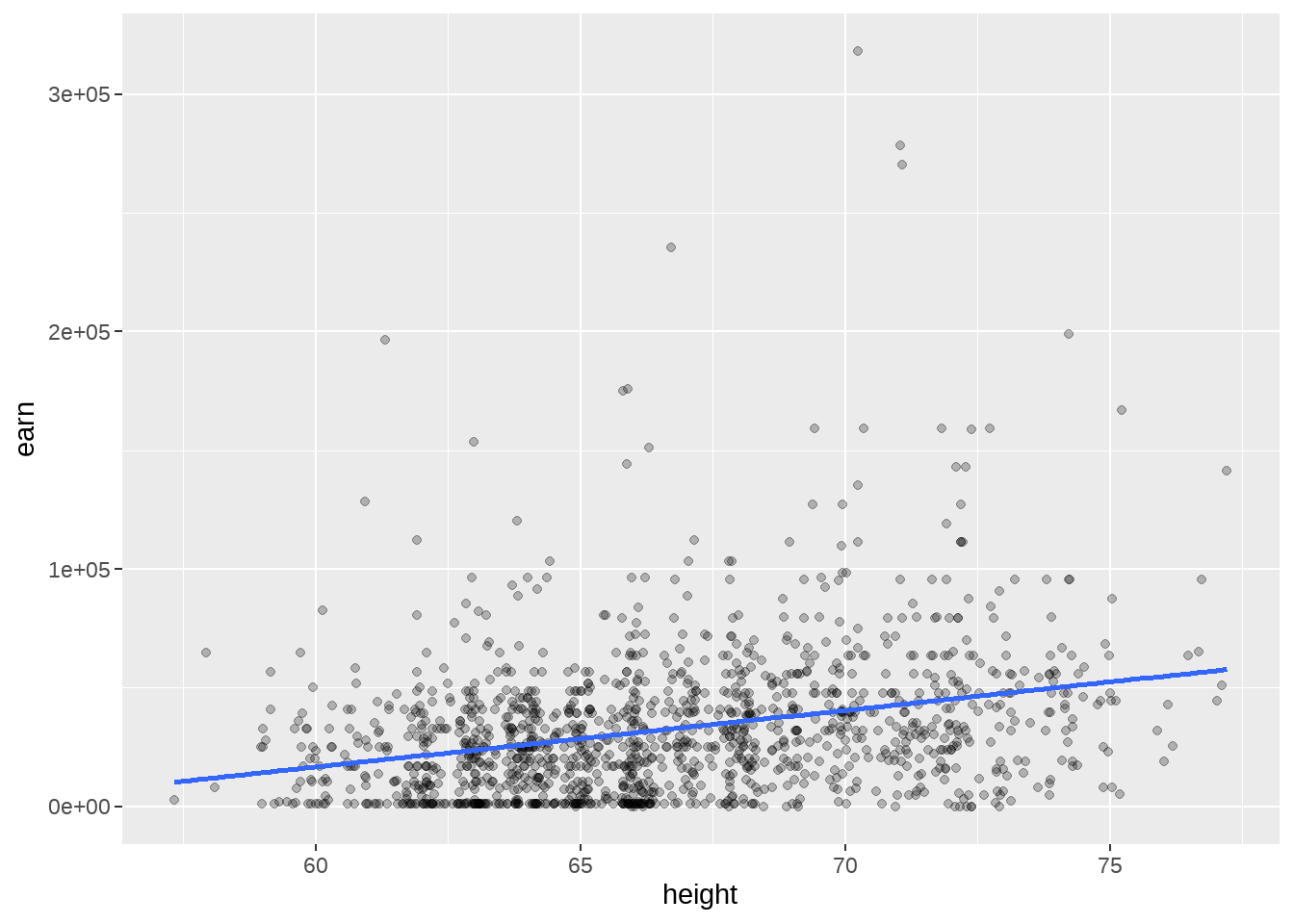
51.5 多元线性回归
刚才讨论的单个预测变量height,现在我们增加一个预测变量ed,稍微扩展一下我们的一元线性模型,就是多元回归模型
\[ \begin{aligned} earn &= \alpha + \beta_1 \text{height} + \beta_2 \text{ed} +\epsilon \\ \end{aligned} \]
R语言代码实现也很简单,只需要把变量ed增加在公式的右边
mod2 <- lm(earn ~ height + ed, data = wages)同样,我们打印mod2看看
mod2##
## Call:
## lm(formula = earn ~ height + ed, data = wages)
##
## Coefficients:
## (Intercept) height ed
## -161541 2087 4118大家试着解释下mod2. 😄
51.6 更多模型
lm(earn ~ sex, data = wages)
lm(earn ~ ed, data = wages)
lm(earn ~ age, data = wages)

lm(earn ~ height + sex, data = wages)
lm(earn ~ height + ed, data = wages)
lm(earn ~ height + age, data = wages)
lm(earn ~ height + race, data = wages)


lm(earn ~ height + sex + ed, data = wages)
lm(earn ~ height + sex + age, data = wages)
lm(earn ~ height + sex + race, data = wages)
lm(earn ~ height + ed + age, data = wages)
lm(earn ~ height + ed + race, data = wages)
lm(earn ~ height + age + race, data = wages)

lm(earn ~ height + sex + ed + age, data = wages)
lm(earn ~ height + sex + ed + race, data = wages)
lm(earn ~ height + sex + age + race, data = wages)
lm(earn ~ height + ed + age + race, data = wages)
lm(earn ~ sex + ed + age + race, data = wages)

lm(earn ~ height + sex + ed + age + race, data = wages)
51.7 变量重要性
哪个变量对收入的影响最大?
lm(earn ~ height + ed + age, data = wages)- 方法一,变量都做标准化处理后,再放到模型中计算,然后对比系数的绝对值
fit <- wages %>%
  mutate_at(vars(earn, height, ed, age), scale) %>%
  lm(earn ~ 1 + height + ed + age, data = .)

summary(fit)
##
## Call:
## lm(formula = earn ~ 1 + height + ed + age, data = .)
##
## Residuals:
## Min 1Q Median 3Q Max
## -1.9213 -0.5356 -0.1206 0.3525 8.2982
##
## Coefficients:
## Estimate Std. Error t value Pr(>|t|)
## (Intercept) -1.768e-16 2.396e-02 0.00 1
## height 2.736e-01 2.430e-02 11.26 < 2e-16 ***
## ed 3.392e-01 2.429e-02 13.97 < 2e-16 ***
## age 1.546e-01 2.435e-02 6.35 2.92e-10 ***
## ---
## Signif. codes: 0 '***' 0.001 '**' 0.01 '*' 0.05 '.' 0.1 ' ' 1
##
## Residual standard error: 0.8897 on 1375 degrees of freedom
## Multiple R-squared: 0.2101, Adjusted R-squared: 0.2084
## F-statistic: 121.9 on 3 and 1375 DF, p-value: < 2.2e-16- 方法二,通过比较模型参数的t-statistic的绝对值,可以考察参数的重要程度
caret::varImp(fit)## Overall
## height 11.257099
## ed 13.965858
## age 6.34978651.8 可能遇到的情形
根据同学们的建议,模型中涉及统计知识,留给统计老师讲,我们这里是R语言课,应该讲代码。 因此,这里再介绍几种线性回归中遇到的几种特殊情况
51.8.2 只有截距项
lm(earn ~ 1, data = wages)##
## Call:
## lm(formula = earn ~ 1, data = wages)
##
## Coefficients:
## (Intercept)
## 32446只有截距项,实质上就是计算y变量的均值
## # A tibble: 1 × 1
##   mean_wages
##        <dbl>
## 1     32446.
51.8.3 分类变量
race变量就是数据框wages的一个分类变量,代表四个不同的种族。用分类变量做回归,本质上是各组之间的进行比较。
## # A tibble: 4 × 1
##   race
##   <chr>
## 1 white
## 2 other
## 3 hispanic
## 4 black
wages %>%
  ggplot(aes(x = race, y = earn, fill = race)) +
  geom_boxplot(position = position_dodge()) +
  scale_y_continuous(limits = c(0, 20000))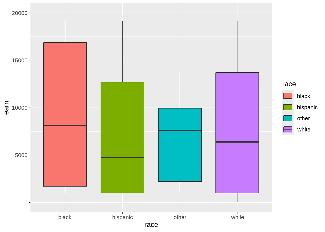
以分类变量作为解释变量,做线性回归
mod3 <- lm(earn ~ race, data = wages)
mod3
##
## Call:
## lm(formula = earn ~ race, data = wages)
##
## Coefficients:
## (Intercept) racehispanic raceother racewhite
## 28372 -2887 3905 4993tidyverse框架下,喜欢数据框的统计结果,因此,可用broom的tidy()函数将模型输出转换为数据框的形式
broom::tidy(mod3)## # A tibble: 4 × 5
## term estimate std.error statistic p.value
## <chr> <dbl> <dbl> <dbl> <dbl>
## 1 (Intercept) 28372. 2781. 10.2 1.29e-23
## 2 racehispanic -2887. 4515. -0.639 5.23e- 1
## 3 raceother 3905. 6428. 0.608 5.44e- 1
## 4 racewhite 4993. 2929. 1.70 8.85e- 2我们看到输出结果,只有race_hispanic、 race_other和race_white三个系数和Intercept截距,race_black去哪里了呢?
事实上,race变量里有4组,回归时,选择black为基线,hispanic的系数,可以理解为由black切换到hispanic,引起earn收入的变化(效应)
- 对 black 组的估计,
earn = 28372.09 = 28372.09 - 对 hispanic组的估计,
earn = 28372.09 + -2886.79 = 25485.30 - 对 other 组的估计,
earn = 28372.09 + 3905.32 = 32277.41 - 对 white 组的估计,
earn = 28372.09 + 4993.33 = 33365.42
分类变量的线性回归本质上就是方差分析
第 54章专题讨论方差分析
51.8.4 因子变量
hispanic组的估计最低,适合做基线,因此可以将race转换为因子变量,这样方便调整因子先后顺序
wages_fct <- wages %>%
  mutate(race = factor(race, levels = c("hispanic", "white", "black", "other"))) %>%
  select(earn, race)

head(wages_fct)
## # A tibble: 6 × 2
## earn race
## <dbl> <fct>
## 1 79571. white
## 2 96397. white
## 3 48711. white
## 4 80478. other
## 5 82089. white
## 6 15313. whitewages_fct替换wages,然后建立线性模型
## # A tibble: 4 × 5
##   term        estimate std.error statistic  p.value
##   <chr>          <dbl>     <dbl>     <dbl>    <dbl>
## 1 (Intercept)   25485.     3557.     7.16  1.26e-12
## 2 racewhite      7880.     3674.     2.14  3.22e- 2
## 3 raceblack      2887.     4515.     0.639 5.23e- 1
## 4 raceother      6792.     6800.     0.999 3.18e- 1
以hispanic组作为基线,各组系数也调整了,但加上截距后,实际值是没有变的。
大家可以用sex变量试试看
lm(earn ~ sex, data = wages)51.8.5 一个分类变量和一个连续变量
如果预测变量是一个分类变量和一个连续变量
## (Intercept)      height     sexmale
## -32479.861 879.424 16874.158-
height = 879.424当sex保持不变时,height变化引起的earn变化 -
sexmale = 16874.158当height保持不变时,sex变化(female变为male)引起的earn变化
p1 <- wages %>%
  ggplot(aes(x = height, y = earn, color = sex)) +
  geom_point(alpha = 0.1) +
  geom_line(aes(y = predict(mod5))) +
  coord_cartesian(ylim = c(0, 100000))
p1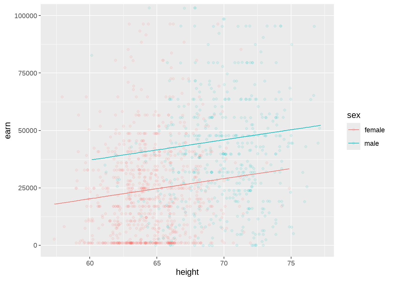
51.8.6 偷懒的写法
. is shorthand for “everything else.”
lm(earn ~ height + sex + race + ed + age, data = wages)
lm(earn ~ ., data = wages)

lm(earn ~ height + sex + race + ed, data = wages)
lm(earn ~ . - age, data = wages)
R 语言很多时候都出现了.,不同的场景,含义是不一样的。我会在后面第 46 章专门讨论这个问题, 这是一个非常重要的问题
51.8.7 交互项
lm(earn ~ height + sex + height:sex, data = wages)
lm(earn ~ height * sex, data = wages)
lm(earn ~ (height + sex)^2, data = wages)## (Intercept) height sexmale height:sexmale
## -12166.9667 564.5102 -30510.4336 701.4065- 对于女性,height增长1个单位,引起earn的增长
564.5102 - 对于男性,height增长1个单位,引起earn的增长
564.5102 + 701.4065 = 1265.92
p2 <- wages %>%
  ggplot(aes(x = height, y = earn, color = sex)) +
  geom_point(alpha = 0.1) +
  geom_line(aes(y = predict(mod6))) +
  coord_cartesian(ylim = c(0, 100000))
p2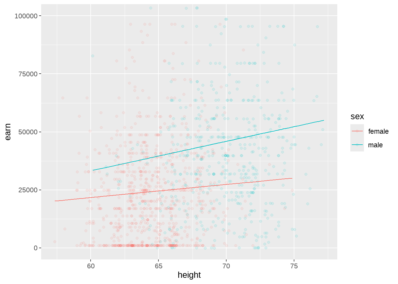
注意,没有相互项和有相互项的区别
library(patchwork)

combined <- p1 + p2 & theme(legend.position = "bottom")
combined + plot_layout(guides = "collect")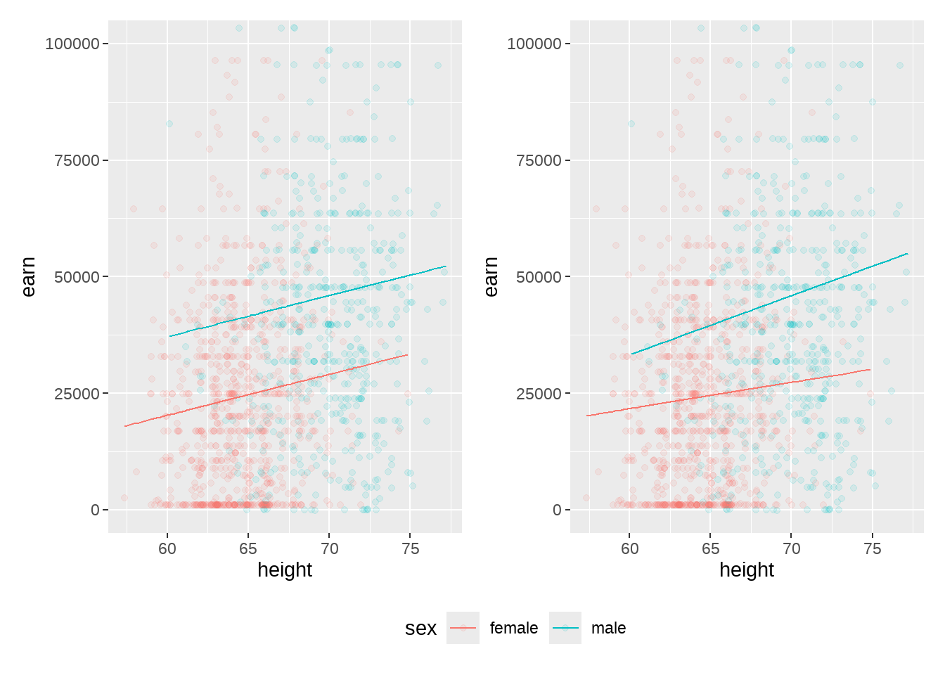
51.8.8 虚拟变量
交互项,有点不好理解?我们再细致说一遍
earn ~ height + sex + height:sex对应的数学表达式 \[ \begin{aligned} \text{earn} &= \alpha + \beta_1 \text{height} + \beta_2 \text{sex} +\beta_3 \text{(height*sex)}+ \epsilon \\ \end{aligned} \]
我们要求出其中的\(\alpha, \beta_1, \beta_2, \beta_3\),事实上,分类变量在R语言代码里,会转换成0和1这种虚拟变量,然后再计算。类似
## # A tibble: 1,379 × 7
##      earn height sex    race        ed   age sexmale
##     <dbl>  <dbl> <chr>  <chr>    <dbl> <dbl>   <dbl>
##  1 79571.   73.9 male   white       16    49       1
##  2 96397.   66.2 female white       16    62       0
##  3 48711.   63.8 female white       16    33       0
##  4 80478.   63.2 female other       16    95       0
##  5 82089.   63.1 female white       17    43       0
##  6 15313.   64.5 female white       15    30       0
##  7 47104.   61.5 female white       12    53       0
##  8 50960.   73.3 male   white       17    50       1
##  9  3213.   72.2 male   hispanic    15    25       1
## 10 42997.   72.4 male   white       12    30       1
## # ℹ 1,369 more rows
那么上面的公式变为 \[ \begin{aligned} \text{earn} &= \alpha + \beta_1 \text{height} + \beta_2 \text{sexmale} +\beta_3 \text{(height*sexmale)}+ \epsilon \\ \end{aligned} \]
于是,可以将上面的公式里男性(sexmale = 1)和女性(sexmale = 0)分别表示
\[
\begin{aligned}
\text{female}\qquad earn &= \alpha + \beta_1 \text{height} +\epsilon \\
\text{male}\qquad earn &= \alpha + \beta_1 \text{height} + \beta_2 *1 +\beta_3 \text{(height*1)}+ \epsilon \\
&= \alpha + \beta_1 \text{height} + \beta_2 +\beta_3 \text{height}+ \epsilon \\
& = (\alpha + \beta_2) + (\beta_1 + \beta_3)\text{height} + \epsilon \\
\end{aligned}
\]
我们再对比mod6结果中的系数\(\alpha, \beta_1, \beta_2, \beta_3\)
mod6##
## Call:
## lm(formula = earn ~ height + sex + height:sex, data = wages)
##
## Coefficients:
## (Intercept) height sexmale height:sexmale
## -12167.0 564.5 -30510.4 701.4是不是更容易理解呢?
- 对于女性,(截距\(\alpha\),系数\(\beta_1\)),height增长1个单位,引起earn的增长
564.5102 - 对于男性,(截距\(\alpha + \beta_2\),系数\(\beta_1 + \beta_3\)),height增长1个单位,引起earn的增长
564.5102 + 701.4065 = 1265.92
事实上,对于男性和女性,截距和系数都不同,因此这种情形等价于,按照sex分成两组,男性算男性的斜率,女性算女性的斜率
## # A tibble: 4 × 6
## # Groups:   sex [2]
##   sex    term        estimate std.error statistic p.value
##   <chr>  <chr>          <dbl>     <dbl>     <dbl>   <dbl>
## 1 female (Intercept)  -12167.    20160.    -0.604  0.546
## 2 female height          565.      312.     1.81   0.0710
## 3 male   (Intercept)  -42677.    38653.    -1.10   0.270
## 4 male   height         1266.      551.     2.30   0.0221
wages %>%
  ggplot(aes(x = height, y = earn, color = sex)) +
  geom_smooth(method = lm, se = F)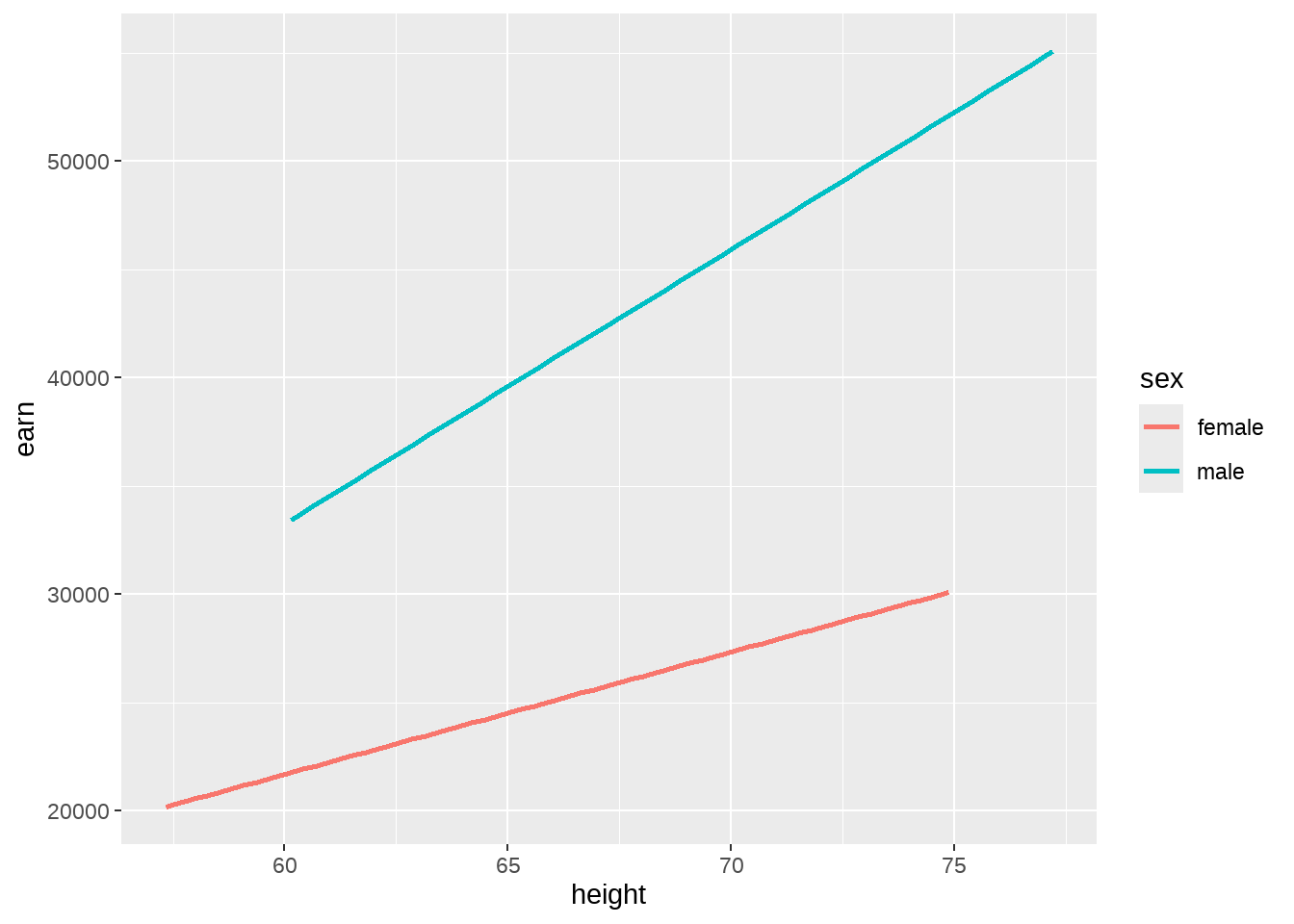
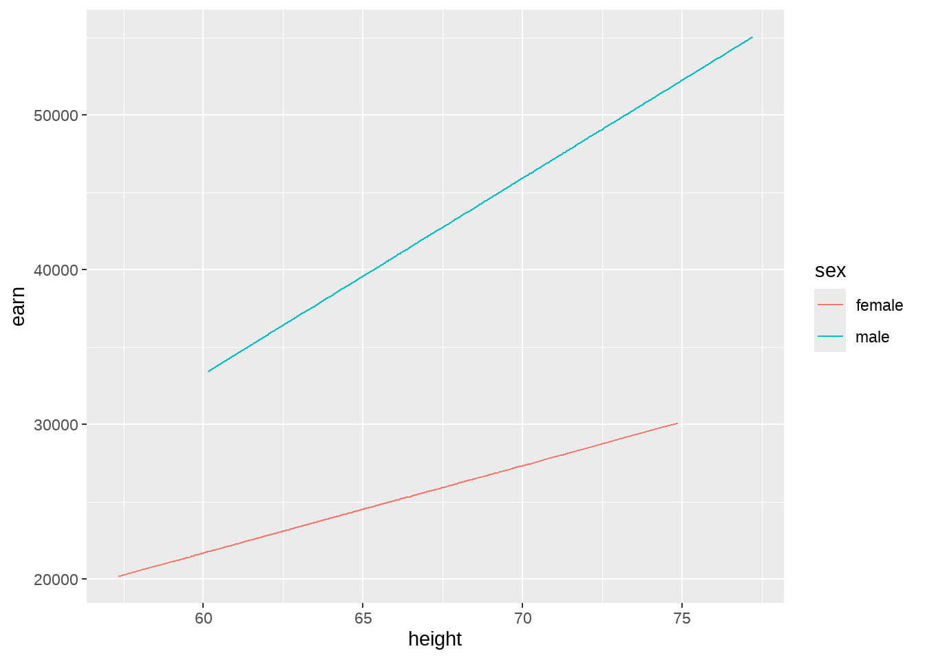
如果再特殊一点的模型(有点过分了)
##    (Intercept)         height height:sexmale
##    -24632.6695       757.4661       251.2915
这又怎么理解呢?
我们还是按照数学模型来理解,这里对应的数学表达式 \[ \begin{aligned} \text{earn} &= \alpha + \beta_1 \text{height} + \beta_4 \text{(height*sex)}+ \epsilon \\ \end{aligned} \]
引入虚拟变量
\[ \begin{aligned} \text{earn} &= \alpha + \beta_1 \text{height} + \beta_4 \text{(height*sexmale)}+ \epsilon \\ \end{aligned} \]
同样假定男性(sexmale = 1)和女性(sexmale = 0),那么 \[ \begin{aligned} \text{female}\qquad earn &= \alpha + \beta_1 \text{height} +\epsilon \\ \text{male}\qquad earn &= \alpha + \beta_1 \text{height} + \beta_4 \text{(height*1)}+ \epsilon \\ &= \alpha + \beta_1 \text{height} + \beta_4 \text{height}+ \epsilon \\ & = \alpha + (\beta_1 + \beta_4)\text{height} + \epsilon \\ \end{aligned} \]
对照模型mod7的结果,我们可以理解:
- 对于女性(截距\(\alpha\),系数\(\beta_1\)),height增长1个单位,引起earn的增长
757.4661 - 对于男性(截距\(\alpha\),系数$_1 + _4 $),height增长1个单位,引起earn的增长
757.4661 + 251.2915 = 1008.758 - 注意到,mod6和mod7是两个不同的模型,
- mod7中男女拟合曲线在y轴的截距是相同的,而mod6在y轴的截距是不同的
51.8.9 predict vs fit
- fitted() , 模型一旦建立,可以使用拟合函数
fitted()返回拟合值,建模和拟合使用的是同一数据 - predict(), 模型建立后,可以用新的数据进行预测,
predict()要求数据框包含新的预测变量,如果没有提供,那么就使用建模时的预测变量进行预测,这种情况下,得出的结果和fitted()就时一回事了。
predict()函数和fitted()函数不同的地方,还在于predict()函数往往带有返回何种类型的选项,可以是具体数值,也可以是分类变量。具体会在第 63 章介绍。
51.9 延伸阅读
一篇极富思考性和启发性的文章《常见统计检验的本质是线性模型》