第 60 章 有序logistic回归

本节课，是广义线性模型的延续

library(tidyverse)

60.1 logistic回归

• 二元logistic回归：Y为定类且为2个，比如是否购买(1购买；0不购买)
• 多分类logistic回归：Y为定类且选项大于2个，比如总统候选人偏好(特朗普、希拉里、卢比奥)
• 有序logistic回归：Y为定类且有序，幸福感(不幸福、比较幸福和非常幸福)

60.2 生活中的有序logistic回归

• 人们在肯德基里点餐，一般都会买可乐，可乐有四种型号(small, medium, large or extra large)，选择何种型号的可乐会与哪些因素有关呢？是否购买了汉堡、是否购买了薯条，消费者的年龄等。我们这里考察的被解释变量，可乐的大小就是一个有序的值。

• 问卷调查。问大三的学生是否申请读研究生，有三个选项：1不愿意，2有点愿意，3非常愿意。那么这里的被解释变量是三个有序的类别，影响读研意愿的因素可能与父母的教育水平、本科阶段学习成绩、经济压力等有关。

60.3 案例

教育代际传递。通俗点说子女的教育程度是否受到父母教育程度的影响。我这个案例思路参考了南京大学池彪的《教育人力资本的代际传递研究》硕士论文，这篇文章思路很清晰，建议大家可以看看。根据文中提供的数据来源，我们下载2016年的中国家庭追踪调查数据CFPS，并整理了部分数据。

tb <- readr::read_rds("./demo_data/cfps.rds")
head(tb)

## # A tibble: 6 × 8
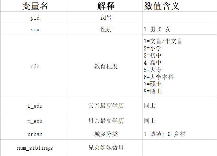
##         pid   sex   age   edu edu_f edu_m urban num_siblings
##       <dbl> <dbl> <dbl> <dbl> <dbl> <dbl> <dbl>        <int>
## 1 101581553     1    28     5     3     2     1            1
## 2 103924503     1    34     6     4     4     1            1
## 3 108660552     1    43     3     1     1     1            1
## 4 109137501     1    31     4     4     4     1            1
## 5 110009107     1    28     6     1     1     1            1
## 6 110020104     1    42     4     2     2     1            1

tb %>% count(edu)

## # A tibble: 8 × 2
##     edu     n
##   <dbl> <int>
## 1     1   399
## 2     2   801
## 3     3  1492
## 4     4   706
## 5     5   475
## 6     6   374
## 7     7    46
## 8     8     2

tb %>% count(edu_f)

## # A tibble: 6 × 2
##   edu_f     n
##   <dbl> <int>
## 1     1  1345
## 2     2  1090
## 3     3  1125
## 4     4   639
## 5     5    72
## 6     6    24

tb %>% count(edu_m)

## # A tibble: 6 × 2
##   edu_m     n
##   <dbl> <int>
## 1     1  2482
## 2     2   768
## 3     3   712
## 4     4   310
## 5     5    17
## 6     6     6

为了方便处理，减少分类，我们将大专以及大专以上的都归为一类

df <- tb %>%
  dplyr::mutate(
    across(
      starts_with("edu"),
      ~ case_when(
        . %in% c(5, 6, 7, 8) ~ 5,
        TRUE ~ .
      )
    )
  )
df

## # A tibble: 4,295 × 8
##          pid   sex   age   edu edu_f edu_m urban num_siblings
##        <dbl> <dbl> <dbl> <dbl> <dbl> <dbl> <dbl>        <int>
##  1 101581553     1    28     5     3     2     1            1
##  2 103924503     1    34     5     4     4     1            1
##  3 108660552     1    43     3     1     1     1            1
##  4 109137501     1    31     4     4     4     1            1
##  5 110009107     1    28     5     1     1     1            1
##  6 110020104     1    42     4     2     2     1            1
##  7 110026102     1    43     5     5     3     1            1
##  8 110043103     1    31     4     4     4     1            2
##  9 110051104     0    30     4     4     4     1            1
## 10 110052104     1    30     5     4     4     1            1
## # ℹ 4,285 more rows

看起很复杂？那我写简单点

tb %>%
  dplyr::mutate(
    across(
      starts_with("edu"),
      ~ if_else(. %in% c(5, 6, 7, 8), 5, .)
    )
  )

## # A tibble: 4,295 × 8
##          pid   sex   age   edu edu_f edu_m urban num_siblings
##        <dbl> <dbl> <dbl> <dbl> <dbl> <dbl> <dbl>        <int>
##  1 101581553     1    28     5     3     2     1            1
##  2 103924503     1    34     5     4     4     1            1
##  3 108660552     1    43     3     1     1     1            1
##  4 109137501     1    31     4     4     4     1            1
##  5 110009107     1    28     5     1     1     1            1
##  6 110020104     1    42     4     2     2     1            1
##  7 110026102     1    43     5     5     3     1            1
##  8 110043103     1    31     4     4     4     1            2
##  9 110051104     0    30     4     4     4     1            1
## 10 110052104     1    30     5     4     4     1            1
## # ℹ 4,285 more rows

df %>% count(edu)

## # A tibble: 5 × 2
##     edu     n
##   <dbl> <int>
## 1     1   399
## 2     2   801
## 3     3  1492
## 4     4   706
## 5     5   897

df %>% count(edu_f)

## # A tibble: 5 × 2
##   edu_f     n
##   <dbl> <int>
## 1     1  1345
## 2     2  1090
## 3     3  1125
## 4     4   639
## 5     5    96

df %>% count(edu_m)

## # A tibble: 5 × 2
##   edu_m     n
##   <dbl> <int>
## 1     1  2482
## 2     2   768
## 3     3   712
## 4     4   310
## 5     5    23

60.4 问题的提出

问题的提出：

• 学历上父母是否门当户对？
• 父母的受教育程度对子女的受教育水平是正向影响？
• 父亲和母亲谁的影响大？
• 对男孩影响大？还是对女孩影响大？
• 以上情况城乡有无差异？

60.4.1 父母门当户对？

数据还是比较有意思的，我们来看看父母是否门当户对

多大比例选择门当户对?

df

## # A tibble: 4,295 × 8
##          pid   sex   age   edu edu_f edu_m urban num_siblings
##        <dbl> <dbl> <dbl> <dbl> <dbl> <dbl> <dbl>        <int>
##  1 101581553     1    28     5     3     2     1            1
##  2 103924503     1    34     5     4     4     1            1
##  3 108660552     1    43     3     1     1     1            1
##  4 109137501     1    31     4     4     4     1            1
##  5 110009107     1    28     5     1     1     1            1
##  6 110020104     1    42     4     2     2     1            1
##  7 110026102     1    43     5     5     3     1            1
##  8 110043103     1    31     4     4     4     1            2
##  9 110051104     0    30     4     4     4     1            1
## 10 110052104     1    30     5     4     4     1            1
## # ℹ 4,285 more rows

df %>%
  dplyr::summarise(
    eq_n = sum(edu_m == edu_f),
    n = n()
  ) %>%
  dplyr::mutate(prop = eq_n / n)

## # A tibble: 1 × 3
##    eq_n     n  prop
##   <int> <int> <dbl>
## 1  1829  4295 0.426

df %>%
  dplyr::count(edu_m, edu_f) %>%
  dplyr::group_by(edu_m) %>%
  dplyr::mutate(prop = n / sum(n)) %>%
  dplyr::ungroup()

## # A tibble: 24 × 4
##    edu_m edu_f     n    prop
##    <dbl> <dbl> <int>   <dbl>
##  1     1     1  1106 0.446  
##  2     1     2   635 0.256  
##  3     1     3   491 0.198  
##  4     1     4   230 0.0927 
##  5     1     5    20 0.00806
##  6     2     1   147 0.191  
##  7     2     2   276 0.359  
##  8     2     3   224 0.292  
##  9     2     4   111 0.145  
## 10     2     5    10 0.0130 
## # ℹ 14 more rows

df %>%
  dplyr::count(edu_m, edu_f) %>%
  dplyr::group_by(edu_m) %>%
  dplyr::mutate(percent = n / sum(n)) %>%
  dplyr::select(-n) %>%
  tidyr::pivot_wider(
    names_from = edu_f,
    values_from = percent
  )

## # A tibble: 5 × 6
## # Groups:   edu_m [5]
##   edu_m    `1`    `2`   `3`    `4`     `5`
##   <dbl>  <dbl>  <dbl> <dbl>  <dbl>   <dbl>
## 1     1 0.446   0.256 0.198 0.0927 0.00806
## 2     2 0.191   0.359 0.292 0.145  0.0130 
## 3     3 0.0927  0.191 0.438 0.233  0.0449 
## 4     4 0.0774  0.139 0.303 0.403  0.0774 
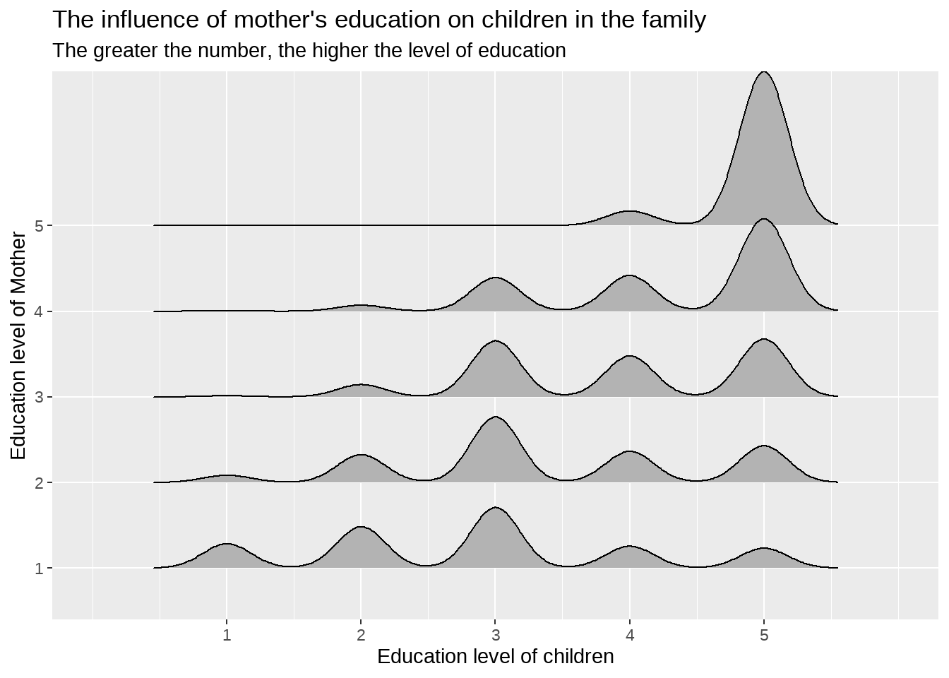
## 5     5 0.0870 NA     0.174 0.304  0.435

60.4.2 母亲的教育程度对子女的影响

library(ggridges)
df %>%
  dplyr::mutate(
    across(edu_m, as.factor)
  ) %>%
  ggplot(aes(x = edu, y = edu_m)) +
  geom_density_ridges() +
  scale_x_continuous(limits = c(0, 6), breaks = c(1:5)) +
  labs(
    title = "The influence of mother's education on children in the family",
    subtitle = "The greater the number, the higher the level of education",
    x = "Education level of children",
    y = "Education level of Mother"
  )

60.4.3 父亲和母亲谁的影响大

这里需要用到有序logistic回归。 为了理解模型的输出，我们需要先简单介绍下模型的含义。假定被解释变量\(Y\)有\(J\)类且有序，那么\(Y\) 小于等于某个具体类别\(j\)的累积概率，可以写为\(P(Y \le j)\)，这里\(j = 1, \cdots, J-1\).

从而，小于等于某个具体类别\(j\)的比率就可以定义为

\[\frac{P(Y \le j)}{P(Y>j)}\] 对这个比率取对数，就是我们熟知的logit

\[log \frac{P(Y \le j)}{P(Y>j)} = logit (P(Y \le j)).\]

，有序logistic回归的数学模型就是

\[logit (P(Y \le j)) = \alpha_{j} + \beta_{1}x_1 + \beta_{2}x_2 \] \(\alpha\) 是截距 \(\beta\) 是回归系数，注意到有序分类 logistic 回归模型中就有 \(J-1\) 个 logit 模型。对于每个模型，系数是相同的，截距不同。

在R语言中，我们可以使用MASS::polr函数，但需要注意的是，使用这个函数，对应的模型表达式为¹¹，斜率符号写为负号

\[logit (P(Y \le j)) = \alpha_{j} - \beta_{1}x_1 - \beta_{2}x_2 \]

下面我们通过代码来演示

library(MASS)
df1 <- df %>%
  dplyr::mutate(
    across(c(edu, sex, urban), as.factor),
    across(edu, ~ fct_inseq(., ordered = TRUE))
  )

mod_mass <- polr(edu ~ edu_f + edu_m + sex + num_siblings + urban,
  data = df1,
  method = c("logistic")
)

summary(mod_mass)

## Call:
## polr(formula = edu ~ edu_f + edu_m + sex + num_siblings + urban, 
##     data = df1, method = c("logistic"))
## 
## Coefficients:
##                Value Std. Error t value
## edu_f         0.4611    0.02836  16.258
## edu_m         0.5074    0.03229  15.715
## sex1         -0.4609    0.06929  -6.652
## num_siblings -0.1540    0.04364  -3.530
## urban1        0.9570    0.06015  15.911
## 
## Intercepts:
##     Value   Std. Error t value
## 1|2 -0.8385  0.1217    -6.8925
## 2|3  0.6742  0.1174     5.7425
## 3|4  2.5093  0.1236    20.2955
## 4|5  3.5454  0.1293    27.4298
## 
## Residual Deviance: 11680.22 
## AIC: 11698.22

输出结果得到有序分类 logistic 回归模型中截距和回归系数的最大似然估计值，确定出回归方程为：

\[ \begin{aligned} \text{logit}(\hat{P}(Y \le 1))&= \text{logit}\left(p_{1}\right) = \ln \left(\frac{p_{1}}{1 - p_{1}}\right) = -0.8385 - 0.46 \times \text{edu_f} - 0.51 \times\text{edu_m} -(-0.46)\times\text{sex1} -(-0.15)\times \text{num_siblings} -0.96 \times\text{urban1} \\ \text{logit}(\hat{P}(Y \le 2))&= \text{logit}\left(p_{1} + p_{2}\right) = \ln \left(\frac{p_{1} + p_{2}}{1 - p_{1} - p_{2}}\right) = 0.6742 - 0.46 \times \text{edu_f} - 0.51 \times\text{edu_m} -(-0.46)\times\text{sex1} -(-0.15)\times \text{num_siblings} -0.96 \times\text{urban1} \\ \text{logit}(\hat{P}(Y \le 3))&= \text{logit}\left(p_{1} + p_{2} + p_{3}\right) = \ln \left(\frac{p_{1} + p_{2} + p_{3}}{1 - p_{1} - p_{2} - p_{3}}\right) = 2.5093 - 0.46 \times \text{edu_f} - 0.51 \times\text{edu_m} -(-0.46)\times\text{sex1} -(-0.15)\times \text{num_siblings} -0.96 \times\text{urban1}\\ \text{logit}(\hat{P}(Y \le 4))&= \text{logit}\left(p_{1} + p_{2} + p_{3} + p_{4}\right) = \ln \left(\frac{p_{1} + p_{2} + p_{3} + p_{4}}{1 - p_{1} - p_{2} - p_{3} - p_{4}}\right) = 3.5454 - 0.46 \times \text{edu_f} - 0.51 \times\text{edu_m} -(-0.46)\times\text{sex1} -(-0.15)\times \text{num_siblings} -0.96 \times\text{urban1}\\ \end{aligned} \]

60.4.4 系数的解释

关于系数的解释，推荐您阅读这里。

先将系数转换成odds ratios(OR)

coef(mod_mass) %>% exp()

##        edu_f        edu_m         sex1 num_siblings       urban1 
##    1.5858540    1.6610310    0.6306987    0.8572473    2.6038469

• 在其它因素不变的情况下，父亲教育程度每增加一个等级（比如，大专到本科）， 会增加子女教育程度向上提高一个级别的概率1.58倍，也就是增加了58%。
• 在其它因素不变的情况下，母亲教育程度每提高一个等级，会增加提升子女教育水平的概率1.66倍.
• 从子女的性别差异来看, 在其它因素不变的情况下，女性的受教育水平向上提高一个级别的概率更大，是男性的(1/0.630)倍，或者说，男性受教育水平向上提高一个级别的概率比女性减少37%(1 - 0.63).
• 从城乡差异来看，城镇子女提升教育水平的概率是农村的2.6倍

60.4.5 边际效应

library(margins)
# me_mass <- marginal_effects(mod_mass, variables = "sex")
me_mass <- marginal_effects(mod_mass, variables = "edu_m")
me_mass %>% 
  head()

##     dydx_edu_m
## 1 -0.013404128
## 2 -0.003196004
## 3 -0.047453030
## 4 -0.003196004
## 5 -0.047453030
## 6 -0.020596503

从边际效应图可以看到，随着父母教育程度的增加，子女低学历的的概率减少，高学历的概率增加

60.5 其他宏包

60.5.1 ordinal 包

library(ordinal)
mod_ordinal <- clm(edu ~ edu_f + edu_m + sex + num_siblings + urban,
  data = df1,
  link = "logit",
  thresholds = "flexible"
)

broom::tidy(mod_ordinal)

## # A tibble: 9 × 6
##   term         estimate std.error statistic   p.value coef.type
##   <chr>           <dbl>     <dbl>     <dbl>     <dbl> <chr>    
## 1 1|2            -0.838    0.122      -6.89 5.48e- 12 intercept
## 2 2|3             0.674    0.117       5.74 9.34e-  9 intercept
## 3 3|4             2.51     0.124      20.3  1.41e- 91 intercept
## 4 4|5             3.55     0.129      27.4  1.21e-165 intercept
## 5 edu_f           0.461    0.0284     16.3  1.98e- 59 location 
## 6 edu_m           0.507    0.0323     15.7  1.19e- 55 location 
## 7 sex1           -0.461    0.0693     -6.65 2.89e- 11 location 
## 8 num_siblings   -0.154    0.0436     -3.53 4.16e-  4 location 
## 9 urban1          0.957    0.0601     15.9  5.30e- 57 location