第 39 章 tidyverse中的列方向和行方向
dplyr宏包是数据科学tidyverse集合的核心部件之一,Hadley Wickham大神说将会在5月15日发布dplyr 1.0版本,欢呼。
为迎接新时代的到来,我在线上同大家一起分享dplyr 1.0版本新的特点和功能,看看都为我们带来哪些惊喜?
39.1 体验新版本
New dplyr - 8 things to know:
- Built in
tidyselect relocate()- Superpowered
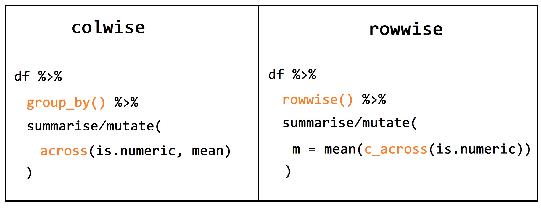
summarise() - colwise using
across() -
cur_data(),cur_group()andcur_column() - new
rowwise()grammar - easy modeling inside dataframes
nest_by()
39.3 summarise()更强大了
在dplyr 1.0之前,summarise()会把统计结果整理成一行一列的数据框,现在可以根据函数返回的结果,可以有多种形式:
- 长度为 1 的向量,比如,
min(x), n(), or sum(is.na(y)) -
长度为 n 的向量,比如,
quantile() - 数据框
df <- tibble(
  grp = rep(c("a", "b"), each = 5),
  x = c(rnorm(5, -0.25, 1), rnorm(5, 0, 1.5)),
  y = c(rnorm(5, 0.25, 1), rnorm(5, 0, 0.5))
)
df
## # A tibble: 10 × 3
## grp x y
## <chr> <dbl> <dbl>
## 1 a -0.712 -0.570
## 2 a -2.01 -0.0256
## 3 a 0.0790 0.460
## 4 a 0.310 0.663
## 5 a -0.630 -1.56
## 6 b 1.46 0.758
## 7 b 0.272 0.771
## 8 b -0.534 -0.0944
## 9 b -1.94 0.271
## 10 b 0.113 0.431## # A tibble: 2 × 2
## grp rng
## <chr> <dbl>
## 1 a -0.594
## 2 b -0.126当统计函数返回多个值的时候,比如range()返回是最小值和最大值,summarise()很贴心地将结果整理成多行,这样符合tidy的格式。
## # A tibble: 4 × 2
## # Groups: grp [2]
## grp rng
## <chr> <dbl>
## 1 a -2.01
## 2 a 0.310
## 3 b -1.94
## 4 b 1.46类似的还有quantile()函数,也是返回多个值
## # A tibble: 6 × 2
## # Groups: grp [2]
## grp rng
## <chr> <dbl>
## 1 a -1.75
## 2 a -0.630
## 3 a 0.264
## 4 b -1.66
## 5 b 0.113
## 6 b 1.23## # A tibble: 6 × 3
## # Groups: grp [2]
## grp x q
## <chr> <dbl> <dbl>
## 1 a -0.712 0.25
## 2 a -0.630 0.5
## 3 a 0.0790 0.75
## 4 b -0.534 0.25
## 5 b 0.113 0.5
## 6 b 0.272 0.75summarise()可以输出数据框,比如
my_quantile <- function(x, probs) {
tibble(x = quantile(x, probs), probs = probs)
}
mtcars %>%
group_by(cyl) %>%
summarise(my_quantile(disp, c(0.25, 0.75)))## # A tibble: 6 × 3
## # Groups: cyl [3]
## cyl x probs
## <dbl> <dbl> <dbl>
## 1 4 78.8 0.25
## 2 4 121. 0.75
## 3 6 160 0.25
## 4 6 196. 0.75
## 5 8 302. 0.25
## 6 8 390 0.75再比如:
dplyr 1.0 之前是需要group_modify()来实现数据框进,数据框出
## # A tibble: 6 × 6
## # Groups: cyl [3]
## cyl term estimate std.error statistic p.value
## <dbl> <chr> <dbl> <dbl> <dbl> <dbl>
## 1 4 (Intercept) 39.6 4.35 9.10 0.00000777
## 2 4 wt -5.65 1.85 -3.05 0.0137
## 3 6 (Intercept) 28.4 4.18 6.79 0.00105
## 4 6 wt -2.78 1.33 -2.08 0.0918
## 5 8 (Intercept) 23.9 3.01 7.94 0.00000405
## 6 8 wt -2.19 0.739 -2.97 0.0118dplyr 1.0 之后,有了新的方案
## # A tibble: 6 × 6
## # Groups: cyl [3]
## cyl term estimate std.error statistic p.value
## <dbl> <chr> <dbl> <dbl> <dbl> <dbl>
## 1 4 (Intercept) 39.6 4.35 9.10 0.00000777
## 2 4 wt -5.65 1.85 -3.05 0.0137
## 3 6 (Intercept) 28.4 4.18 6.79 0.00105
## 4 6 wt -2.78 1.33 -2.08 0.0918
## 5 8 (Intercept) 23.9 3.01 7.94 0.00000405
## 6 8 wt -2.19 0.739 -2.97 0.011839.4 summarise()后的分组信息是去是留?
当 group_by()与summarise()配合使用的时候,summarise()默认会抵消掉最近一次的分组信息,比如下面按照cyl和vs分组,但summarise()后,就只剩下cyl的分组信息了。
## # A tibble: 5 × 3
## # Groups: cyl [3]
## cyl vs cyl_n
## <dbl> <dbl> <int>
## 1 4 0 1
## 2 4 1 10
## 3 6 0 3
## 4 6 1 4
## 5 8 0 14## [1] "cyl"如果想保留vs的分组信息,就需要设置.groups = keep参数
## [1] "cyl" "vs"当然summarise()可以控制输出的更多形式
- 丢弃所有的分组信息
## character(0)- 变成行方向分组,即,每行是一个分组
## [1] "cyl" "vs"39.5 选择某列
- 通过位置索引进行选取
## # A tibble: 10 × 2
## grp y
## <chr> <dbl>
## 1 a -0.570
## 2 a -0.0256
## 3 a 0.460
## 4 a 0.663
## 5 a -1.56
## 6 b 0.758
## 7 b 0.771
## 8 b -0.0944
## 9 b 0.271
## 10 b 0.431## # A tibble: 10 × 2
## x y
## <dbl> <dbl>
## 1 -0.712 -0.570
## 2 -2.01 -0.0256
## 3 0.0790 0.460
## 4 0.310 0.663
## 5 -0.630 -1.56
## 6 1.46 0.758
## 7 0.272 0.771
## 8 -0.534 -0.0944
## 9 -1.94 0.271
## 10 0.113 0.431- 通过列名
## # A tibble: 10 × 3
##    grp         x       y
##    <chr>   <dbl>   <dbl>
##  1 a     -0.712  -0.570
##  2 a     -2.01   -0.0256
##  3 a      0.0790  0.460
##  4 a      0.310   0.663
##  5 a     -0.630  -1.56
##  6 b      1.46    0.758
##  7 b      0.272   0.771
##  8 b     -0.534  -0.0944
##  9 b     -1.94    0.271
## 10 b 0.113 0.431## # A tibble: 10 × 2
## x y
## <dbl> <dbl>
## 1 -0.712 -0.570
## 2 -2.01 -0.0256
## 3 0.0790 0.460
## 4 0.310 0.663
## 5 -0.630 -1.56
## 6 1.46 0.758
## 7 0.272 0.771
## 8 -0.534 -0.0944
## 9 -1.94 0.271
## 10 0.113 0.431- 通过函数选取
df %>% select(starts_with("x"))## # A tibble: 10 × 1
## x
## <dbl>
## 1 -0.712
## 2 -2.01
## 3 0.0790
## 4 0.310
## 5 -0.630
## 6 1.46
## 7 0.272
## 8 -0.534
## 9 -1.94
## 10 0.113## # A tibble: 10 × 1
## grp
## <chr>
## 1 a
## 2 a
## 3 a
## 4 a
## 5 a
## 6 b
## 7 b
## 8 b
## 9 b
## 10 b## # A tibble: 10 × 1
## x
## <dbl>
## 1 -0.712
## 2 -2.01
## 3 0.0790
## 4 0.310
## 5 -0.630
## 6 1.46
## 7 0.272
## 8 -0.534
## 9 -1.94
## 10 0.113## # A tibble: 10 × 1
## x
## <dbl>
## 1 -0.712
## 2 -2.01
## 3 0.0790
## 4 0.310
## 5 -0.630
## 6 1.46
## 7 0.272
## 8 -0.534
## 9 -1.94
## 10 0.113- 通过类型
## # A tibble: 10 × 1
## grp
## <chr>
## 1 a
## 2 a
## 3 a
## 4 a
## 5 a
## 6 b
## 7 b
## 8 b
## 9 b
## 10 b## # A tibble: 10 × 2
## x y
## <dbl> <dbl>
## 1 -0.712 -0.570
## 2 -2.01 -0.0256
## 3 0.0790 0.460
## 4 0.310 0.663
## 5 -0.630 -1.56
## 6 1.46 0.758
## 7 0.272 0.771
## 8 -0.534 -0.0944
## 9 -1.94 0.271
## 10 0.113 0.431- 通过各种组合
## # A tibble: 10 × 2
## x y
## <dbl> <dbl>
## 1 -0.712 -0.570
## 2 -2.01 -0.0256
## 3 0.0790 0.460
## 4 0.310 0.663
## 5 -0.630 -1.56
## 6 1.46 0.758
## 7 0.272 0.771
## 8 -0.534 -0.0944
## 9 -1.94 0.271
## 10 0.113 0.431
df %>% select(where(is.numeric) & starts_with("x"))## # A tibble: 10 × 1
## x
## <dbl>
## 1 -0.712
## 2 -2.01
## 3 0.0790
## 4 0.310
## 5 -0.630
## 6 1.46
## 7 0.272
## 8 -0.534
## 9 -1.94
## 10 0.113
df %>% select(starts_with("g") | ends_with("y"))## # A tibble: 10 × 2
## grp y
## <chr> <dbl>
## 1 a -0.570
## 2 a -0.0256
## 3 a 0.460
## 4 a 0.663
## 5 a -1.56
## 6 b 0.758
## 7 b 0.771
## 8 b -0.0944
## 9 b 0.271
## 10 b 0.431注意any_of和all_of的区别
39.6 重命名某列
## # A tibble: 10 × 3
## group x y
## <chr> <dbl> <dbl>
## 1 a -0.712 -0.570
## 2 a -2.01 -0.0256
## 3 a 0.0790 0.460
## 4 a 0.310 0.663
## 5 a -0.630 -1.56
## 6 b 1.46 0.758
## 7 b 0.272 0.771
## 8 b -0.534 -0.0944
## 9 b -1.94 0.271
## 10 b 0.113 0.431
df %>% rename_with(toupper)## # A tibble: 10 × 3
## GRP X Y
## <chr> <dbl> <dbl>
## 1 a -0.712 -0.570
## 2 a -2.01 -0.0256
## 3 a 0.0790 0.460
## 4 a 0.310 0.663
## 5 a -0.630 -1.56
## 6 b 1.46 0.758
## 7 b 0.272 0.771
## 8 b -0.534 -0.0944
## 9 b -1.94 0.271
## 10 b 0.113 0.431
df %>% rename_with(toupper, is.numeric)## # A tibble: 10 × 3
## grp X Y
## <chr> <dbl> <dbl>
## 1 a -0.712 -0.570
## 2 a -2.01 -0.0256
## 3 a 0.0790 0.460
## 4 a 0.310 0.663
## 5 a -0.630 -1.56
## 6 b 1.46 0.758
## 7 b 0.272 0.771
## 8 b -0.534 -0.0944
## 9 b -1.94 0.271
## 10 b 0.113 0.431
df %>% rename_with(toupper, starts_with("x"))## # A tibble: 10 × 3
## grp X y
## <chr> <dbl> <dbl>
## 1 a -0.712 -0.570
## 2 a -2.01 -0.0256
## 3 a 0.0790 0.460
## 4 a 0.310 0.663
## 5 a -0.630 -1.56
## 6 b 1.46 0.758
## 7 b 0.272 0.771
## 8 b -0.534 -0.0944
## 9 b -1.94 0.271
## 10 b 0.113 0.43139.7 调整列的位置
我们前面一章讲过arrange()排序,这是行方向的排序, 比如按照x变量绝对值的大小从高到低排序。
## # A tibble: 10 × 3
## grp x y
## <chr> <dbl> <dbl>
## 1 a -2.01 -0.0256
## 2 b -1.94 0.271
## 3 b 1.46 0.758
## 4 a -0.712 -0.570
## 5 a -0.630 -1.56
## 6 b -0.534 -0.0944
## 7 a 0.310 0.663
## 8 b 0.272 0.771
## 9 b 0.113 0.431
## 10 a 0.0790 0.460我们现在想调整列的位置,比如,这里调整数据框三列的位置,让grp列放在x列的后面
## # A tibble: 10 × 3
## x grp y
## <dbl> <chr> <dbl>
## 1 -0.712 a -0.570
## 2 -2.01 a -0.0256
## 3 0.0790 a 0.460
## 4 0.310 a 0.663
## 5 -0.630 a -1.56
## 6 1.46 b 0.758
## 7 0.272 b 0.771
## 8 -0.534 b -0.0944
## 9 -1.94 b 0.271
## 10 0.113 b 0.431如果列变量很多的时候,上面的方法就不太好用,因此推荐大家使用relocate()
## # A tibble: 10 × 3
## x y grp
## <dbl> <dbl> <chr>
## 1 -0.712 -0.570 a
## 2 -2.01 -0.0256 a
## 3 0.0790 0.460 a
## 4 0.310 0.663 a
## 5 -0.630 -1.56 a
## 6 1.46 0.758 b
## 7 0.272 0.771 b
## 8 -0.534 -0.0944 b
## 9 -1.94 0.271 b
## 10 0.113 0.431 b## # A tibble: 10 × 3
## x grp y
## <dbl> <chr> <dbl>
## 1 -0.712 a -0.570
## 2 -2.01 a -0.0256
## 3 0.0790 a 0.460
## 4 0.310 a 0.663
## 5 -0.630 a -1.56
## 6 1.46 b 0.758
## 7 0.272 b 0.771
## 8 -0.534 b -0.0944
## 9 -1.94 b 0.271
## 10 0.113 b 0.431还有
## # A tibble: 10 × 3
## x y grp
## <dbl> <dbl> <chr>
## 1 -0.712 -0.570 a
## 2 -2.01 -0.0256 a
## 3 0.0790 0.460 a
## 4 0.310 0.663 a
## 5 -0.630 -1.56 a
## 6 1.46 0.758 b
## 7 0.272 0.771 b
## 8 -0.534 -0.0944 b
## 9 -1.94 0.271 b
## 10 0.113 0.431 b39.8 强大的across函数
我们必须为这个函数点赞。大爱Hadley Wickham !!!
我们经常需要对数据框的多列执行相同的操作。比如
## # A tibble: 150 × 5
## Sepal.Length Sepal.Width Petal.Length Petal.Width Species
## <dbl> <dbl> <dbl> <dbl> <fct>
## 1 5.1 3.5 1.4 0.2 setosa
## 2 4.9 3 1.4 0.2 setosa
## 3 4.7 3.2 1.3 0.2 setosa
## 4 4.6 3.1 1.5 0.2 setosa
## 5 5 3.6 1.4 0.2 setosa
## 6 5.4 3.9 1.7 0.4 setosa
## 7 4.6 3.4 1.4 0.3 setosa
## 8 5 3.4 1.5 0.2 setosa
## 9 4.4 2.9 1.4 0.2 setosa
## 10 4.9 3.1 1.5 0.1 setosa
## # ℹ 140 more rows
iris %>%
group_by(Species) %>%
summarise(
mean_Sepal_Length = mean(Sepal.Length),
mean_Sepal_Width = mean(Sepal.Width),
mean_Petal_Length = mean(Petal.Length),
mean_Petal_Width = mean(Petal.Width)
)## # A tibble: 3 × 5
## Species mean_Sepal_Length mean_Sepal_Width mean_Petal_Length mean_Petal_Width
## <fct> <dbl> <dbl> <dbl> <dbl>
## 1 setosa 5.01 3.43 1.46 0.246
## 2 versico… 5.94 2.77 4.26 1.33
## 3 virgini… 6.59 2.97 5.55 2.03dplyr 1.0之后,使用across()函数异常简练
## # A tibble: 3 × 5
## Species Sepal.Length Sepal.Width Petal.Length Petal.Width
## <fct> <dbl> <dbl> <dbl> <dbl>
## 1 setosa 5.01 3.43 1.46 0.246
## 2 versicolor 5.94 2.77 4.26 1.33
## 3 virginica 6.59 2.97 5.55 2.03或者更科学的
## # A tibble: 3 × 5
## Species Sepal.Length Sepal.Width Petal.Length Petal.Width
## <fct> <dbl> <dbl> <dbl> <dbl>
## 1 setosa 5.01 3.43 1.46 0.246
## 2 versicolor 5.94 2.77 4.26 1.33
## 3 virginica 6.59 2.97 5.55 2.03可以看到,以往是一列一列的处理,现在对多列同时操作,这主要得益于across()函数,它有两个主要的参数:
across(.cols = , .fns = )- 第一个参数.cols,选取我们要需要的若干列,选取多列的语法与
select()的语法一致 - 第二个参数.fns,我们要执行的函数(或者多个函数),函数的语法有三种形式可选:
- A function, e.g. mean.
- A purrr-style lambda, e.g. ~ mean(.x, na.rm = TRUE)
- A list of functions/lambdas, e.g. list(mean = mean, n_miss = ~ sum(is.na(.x))
再看看这个案例
std <- function(x) {
(x - mean(x)) / sd(x)
}
iris %>%
group_by(Species) %>%
summarise(
across(starts_with("Sepal"), std)
)## # A tibble: 150 × 3
## # Groups: Species [3]
## Species Sepal.Length Sepal.Width
## <fct> <dbl> <dbl>
## 1 setosa 0.267 0.190
## 2 setosa -0.301 -1.13
## 3 setosa -0.868 -0.601
## 4 setosa -1.15 -0.865
## 5 setosa -0.0170 0.454
## 6 setosa 1.12 1.25
## 7 setosa -1.15 -0.0739
## 8 setosa -0.0170 -0.0739
## 9 setosa -1.72 -1.39
## 10 setosa -0.301 -0.865
## # ℹ 140 more rows
# purrr style
iris %>%
group_by(Species) %>%
summarise(
across(starts_with("Sepal"), ~ (.x - mean(.x)) / sd(.x))
)## # A tibble: 150 × 3
## # Groups: Species [3]
## Species Sepal.Length Sepal.Width
## <fct> <dbl> <dbl>
## 1 setosa 0.267 0.190
## 2 setosa -0.301 -1.13
## 3 setosa -0.868 -0.601
## 4 setosa -1.15 -0.865
## 5 setosa -0.0170 0.454
## 6 setosa 1.12 1.25
## 7 setosa -1.15 -0.0739
## 8 setosa -0.0170 -0.0739
## 9 setosa -1.72 -1.39
## 10 setosa -0.301 -0.865
## # ℹ 140 more rows
iris %>%
group_by(Species) %>%
summarise(
across(starts_with("Petal"), list(min = min, max = max))
# across(starts_with("Petal"), list(min = min, max = max), .names = "{fn}_{col}")
)## # A tibble: 3 × 5
## Species Petal.Length_min Petal.Length_max Petal.Width_min Petal.Width_max
## <fct> <dbl> <dbl> <dbl> <dbl>
## 1 setosa 1 1.9 0.1 0.6
## 2 versicolor 3 5.1 1 1.8
## 3 virginica 4.5 6.9 1.4 2.5
iris %>%
group_by(Species) %>%
summarise(
across(starts_with("Sepal"), mean),
Area = mean(Petal.Length * Petal.Width),
across(c(Petal.Width), min),
n = n()
)## # A tibble: 3 × 6
## Species Sepal.Length Sepal.Width Area Petal.Width n
## <fct> <dbl> <dbl> <dbl> <dbl> <int>
## 1 setosa 5.01 3.43 0.366 0.1 50
## 2 versicolor 5.94 2.77 5.72 1 50
## 3 virginica 6.59 2.97 11.3 1.4 50除了在summarise()里可以使用外,在其它函数也是可以使用的
## # A tibble: 150 × 5
## Sepal.Length Sepal.Width Petal.Length Petal.Width Species
## <dbl> <dbl> <dbl> <dbl> <fct>
## 1 5.84 3.06 3.76 1.20 setosa
## 2 5.84 3.06 3.76 1.20 setosa
## 3 5.84 3.06 3.76 1.20 setosa
## 4 5.84 3.06 3.76 1.20 setosa
## 5 5.84 3.06 3.76 1.20 setosa
## 6 5.84 3.06 3.76 1.20 setosa
## 7 5.84 3.06 3.76 1.20 setosa
## 8 5.84 3.06 3.76 1.20 setosa
## 9 5.84 3.06 3.76 1.20 setosa
## 10 5.84 3.06 3.76 1.20 setosa
## # ℹ 140 more rows
iris %>% mutate(across(starts_with("Sepal"), mean))## # A tibble: 150 × 5
## Sepal.Length Sepal.Width Petal.Length Petal.Width Species
## <dbl> <dbl> <dbl> <dbl> <fct>
## 1 5.84 3.06 1.4 0.2 setosa
## 2 5.84 3.06 1.4 0.2 setosa
## 3 5.84 3.06 1.3 0.2 setosa
## 4 5.84 3.06 1.5 0.2 setosa
## 5 5.84 3.06 1.4 0.2 setosa
## 6 5.84 3.06 1.7 0.4 setosa
## 7 5.84 3.06 1.4 0.3 setosa
## 8 5.84 3.06 1.5 0.2 setosa
## 9 5.84 3.06 1.4 0.2 setosa
## 10 5.84 3.06 1.5 0.1 setosa
## # ℹ 140 more rows## # A tibble: 150 × 5
## Sepal.Length Sepal.Width Petal.Length Petal.Width Species
## <dbl> <dbl> <dbl> <dbl> <fct>
## 1 -0.898 1.02 -1.34 -1.31 setosa
## 2 -1.14 -0.132 -1.34 -1.31 setosa
## 3 -1.38 0.327 -1.39 -1.31 setosa
## 4 -1.50 0.0979 -1.28 -1.31 setosa
## 5 -1.02 1.25 -1.34 -1.31 setosa
## 6 -0.535 1.93 -1.17 -1.05 setosa
## 7 -1.50 0.786 -1.34 -1.18 setosa
## 8 -1.02 0.786 -1.28 -1.31 setosa
## 9 -1.74 -0.361 -1.34 -1.31 setosa
## 10 -1.14 0.0979 -1.28 -1.44 setosa
## # ℹ 140 more rows
iris %>% mutate(
across(is.numeric, ~ .x / 2),
across(is.factor, stringr::str_to_upper)
)## # A tibble: 150 × 5
## Sepal.Length Sepal.Width Petal.Length Petal.Width Species
## <dbl> <dbl> <dbl> <dbl> <chr>
## 1 2.55 1.75 0.7 0.1 SETOSA
## 2 2.45 1.5 0.7 0.1 SETOSA
## 3 2.35 1.6 0.65 0.1 SETOSA
## 4 2.3 1.55 0.75 0.1 SETOSA
## 5 2.5 1.8 0.7 0.1 SETOSA
## 6 2.7 1.95 0.85 0.2 SETOSA
## 7 2.3 1.7 0.7 0.15 SETOSA
## 8 2.5 1.7 0.75 0.1 SETOSA
## 9 2.2 1.45 0.7 0.1 SETOSA
## 10 2.45 1.55 0.75 0.05 SETOSA
## # ℹ 140 more rows39.9 “current” group or “current” variable
-
n(), 返回当前分组的多少行 -
cur_data(), 返回当前分组的数据内容(不包含分组变量) -
cur_group(), 返回当前分组的分组变量(一行一列的数据框) -
across(cur_column()), 返回当前列的列名
这些函数返回当前分组的信息,因此只能在特定函数内部使用,比如summarise() and mutate()
## # A tibble: 6 × 3
## g x y
## <chr> <dbl> <dbl>
## 1 b 0.0268 0.711
## 2 b 0.549 0.460
## 3 a 0.0351 0.183
## 4 c 0.191 0.634
## 5 c 0.411 0.735
## 6 c 0.340 0.566## # A tibble: 3 × 2
## g n
## <chr> <int>
## 1 a 1
## 2 b 2
## 3 c 3## # A tibble: 3 × 2
## g data
## <chr> <list>
## 1 a <tibble [1 × 1]>
## 2 b <tibble [1 × 1]>
## 3 c <tibble [1 × 1]>## # A tibble: 3 × 2
## g data
## <chr> <list>
## 1 a <tibble [1 × 2]>
## 2 b <tibble [2 × 2]>
## 3 c <tibble [3 × 2]>## # A tibble: 6 × 6
## # Groups: cyl [3]
## cyl term estimate std.error statistic p.value
## <dbl> <chr> <dbl> <dbl> <dbl> <dbl>
## 1 4 (Intercept) 39.6 4.35 9.10 0.00000777
## 2 4 wt -5.65 1.85 -3.05 0.0137
## 3 6 (Intercept) 28.4 4.18 6.79 0.00105
## 4 6 wt -2.78 1.33 -2.08 0.0918
## 5 8 (Intercept) 23.9 3.01 7.94 0.00000405
## 6 8 wt -2.19 0.739 -2.97 0.0118
df %>%
group_by(g) %>%
mutate(across(everything(), ~ paste(cur_column(), round(.x, 2))))## # A tibble: 6 × 3
## # Groups: g [3]
## g x y
## <chr> <chr> <chr>
## 1 b x 0.03 y 0.71
## 2 b x 0.55 y 0.46
## 3 a x 0.04 y 0.18
## 4 c x 0.19 y 0.63
## 5 c x 0.41 y 0.73
## 6 c x 0.34 y 0.57## # A tibble: 6 × 3
## g x y
## <chr> <dbl> <dbl>
## 1 b 0.00536 0.569
## 2 b 0.110 0.368
## 3 a 0.00703 0.146
## 4 c 0.0382 0.507
## 5 c 0.0822 0.588
## 6 c 0.0680 0.45339.10 行方向操作
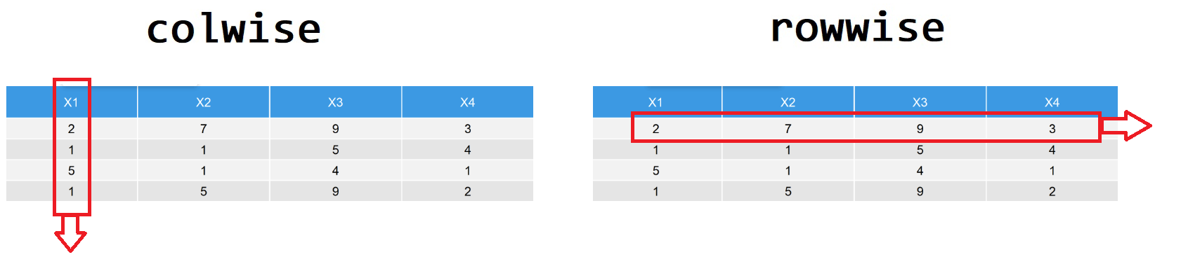
tidyverse遵循的tidy原则,一列表示一个变量,一行表示一次观察。 这种数据的存储格式,对ggplot2很方便,但对行方向的操作或者运算不友好。比如
39.10.1 行方向上的统计
df <- tibble(id = letters[1:6], w = 10:15, x = 20:25, y = 30:35, z = 40:45)
df## # A tibble: 6 × 5
## id w x y z
## <chr> <int> <int> <int> <int>
## 1 a 10 20 30 40
## 2 b 11 21 31 41
## 3 c 12 22 32 42
## 4 d 13 23 33 43
## 5 e 14 24 34 44
## 6 f 15 25 35 45计算每行的均值,
## # A tibble: 6 × 6
## id w x y z avg
## <chr> <int> <int> <int> <int> <dbl>
## 1 a 10 20 30 40 27.5
## 2 b 11 21 31 41 27.5
## 3 c 12 22 32 42 27.5
## 4 d 13 23 33 43 27.5
## 5 e 14 24 34 44 27.5
## 6 f 15 25 35 45 27.5好像不对?为什么呢?
- 按照tidy的方法
df %>%
pivot_longer(
cols = -id,
names_to = "variable",
values_to = "value"
) %>%
group_by(id) %>%
summarize(
r_mean = mean(value)
)## # A tibble: 6 × 2
## id r_mean
## <chr> <dbl>
## 1 a 25
## 2 b 26
## 3 c 27
## 4 d 28
## 5 e 29
## 6 f 30如果保留原始数据,就还需要再left_join()一次,虽然思路清晰,但还是挺周转的。
- 按照Jenny Bryan的方案,使用
purrr宏包的pmap_dbl函数
## # A tibble: 6 × 6
## id w x y z r_mean
## <chr> <int> <int> <int> <int> <dbl>
## 1 a 10 20 30 40 25
## 2 b 11 21 31 41 26
## 3 c 12 22 32 42 27
## 4 d 13 23 33 43 28
## 5 e 14 24 34 44 29
## 6 f 15 25 35 45 30但需要学习新的语法,代价也很高。
## # A tibble: 6 × 6
## # Rowwise:
## id w x y z avg
## <chr> <int> <int> <int> <int> <dbl>
## 1 a 10 20 30 40 25
## 2 b 11 21 31 41 26
## 3 c 12 22 32 42 27
## 4 d 13 23 33 43 28
## 5 e 14 24 34 44 29
## 6 f 15 25 35 45 30变量名要是很多的话,又变了体力活了,怎么才能变的轻巧一点呢?
-
rowwise() + c_across(),现在dplyr 1.0终于给出了一个很好的解决方案
## # A tibble: 6 × 6
## # Rowwise:
## id w x y z avg
## <chr> <int> <int> <int> <int> <dbl>
## 1 a 10 20 30 40 25
## 2 b 11 21 31 41 26
## 3 c 12 22 32 42 27
## 4 d 13 23 33 43 28
## 5 e 14 24 34 44 29
## 6 f 15 25 35 45 30这个很好的解决方案中,rowwise()工作原理类似与group_by(),是按每一行进行分组,然后按行(行方向)统计
## # A tibble: 6 × 6
## # Rowwise: id
## id w x y z total
## <chr> <int> <int> <int> <int> <dbl>
## 1 a 10 20 30 40 25
## 2 b 11 21 31 41 26
## 3 c 12 22 32 42 27
## 4 d 13 23 33 43 28
## 5 e 14 24 34 44 29
## 6 f 15 25 35 45 30## # A tibble: 6 × 6
## # Rowwise: id
## id w x y z mean
## <chr> <int> <int> <int> <int> <dbl>
## 1 a 10 20 30 40 25
## 2 b 11 21 31 41 26
## 3 c 12 22 32 42 27
## 4 d 13 23 33 43 28
## 5 e 14 24 34 44 29
## 6 f 15 25 35 45 30## # A tibble: 6 × 2
## # Groups: id [6]
## id m
## <chr> <dbl>
## 1 a 25
## 2 b 26
## 3 c 27
## 4 d 28
## 5 e 29
## 6 f 30因此,我们可以总结成下面这张图
39.10.2 行方向处理与列表列是天然一对
rowwise()不仅仅用于计算行方向均值这样的简单统计,而是当处理列表列时,方才显示出rowwise()与purrr::map一样的强大。那么,什么是列表列?
列表列指的是数据框的一列是一个列表, 比如
如果想显示列表中每个元素的长度,用purrr包,可以这样写
## # A tibble: 3 × 2
## x l
## <list> <int>
## 1 <dbl [1]> 1
## 2 <int [2]> 2
## 3 <int [3]> 3如果从行方向的角度理解,其实很简练
## # A tibble: 3 × 2
## # Rowwise:
## x l
## <list> <int>
## 1 <dbl [1]> 1
## 2 <int [2]> 2
## 3 <int [3]> 339.10.3 行方向上的建模
## # A tibble: 32 × 11
## mpg cyl disp hp drat wt qsec vs am gear carb
## <dbl> <dbl> <dbl> <dbl> <dbl> <dbl> <dbl> <dbl> <dbl> <dbl> <dbl>
## 1 21 6 160 110 3.9 2.62 16.5 0 1 4 4
## 2 21 6 160 110 3.9 2.88 17.0 0 1 4 4
## 3 22.8 4 108 93 3.85 2.32 18.6 1 1 4 1
## 4 21.4 6 258 110 3.08 3.22 19.4 1 0 3 1
## 5 18.7 8 360 175 3.15 3.44 17.0 0 0 3 2
## 6 18.1 6 225 105 2.76 3.46 20.2 1 0 3 1
## 7 14.3 8 360 245 3.21 3.57 15.8 0 0 3 4
## 8 24.4 4 147. 62 3.69 3.19 20 1 0 4 2
## 9 22.8 4 141. 95 3.92 3.15 22.9 1 0 4 2
## 10 19.2 6 168. 123 3.92 3.44 18.3 1 0 4 4
## # ℹ 22 more rows以cyl分组,计算每组中mpg ~ wt的线性模型的系数.
## # A tibble: 3 × 2
## # Groups: cyl [3]
## cyl data
## <dbl> <list>
## 1 6 <tibble [7 × 10]>
## 2 4 <tibble [11 × 10]>
## 3 8 <tibble [14 × 10]>39.10.3.1 列方向的做法
分组建模后,形成列表列,此时列表中的每个元素对应一个模型,我们需要依次提取每次模型的系数,列方向的做法是,借用purrr::map完成列表中每个模型的迭代,
mtcars %>%
group_by(cyl) %>%
nest() %>%
mutate(model = purrr::map(data, ~ lm(mpg ~ wt, data = .))) %>%
mutate(result = purrr::map(model, ~ broom::tidy(.))) %>%
unnest(result)## # A tibble: 6 × 8
## # Groups: cyl [3]
## cyl data model term estimate std.error statistic p.value
## <dbl> <list> <list> <chr> <dbl> <dbl> <dbl> <dbl>
## 1 6 <tibble [7 × 10]> <lm> (Interce… 28.4 4.18 6.79 1.05e-3
## 2 6 <tibble [7 × 10]> <lm> wt -2.78 1.33 -2.08 9.18e-2
## 3 4 <tibble [11 × 10]> <lm> (Interce… 39.6 4.35 9.10 7.77e-6
## 4 4 <tibble [11 × 10]> <lm> wt -5.65 1.85 -3.05 1.37e-2
## 5 8 <tibble [14 × 10]> <lm> (Interce… 23.9 3.01 7.94 4.05e-6
## 6 8 <tibble [14 × 10]> <lm> wt -2.19 0.739 -2.97 1.18e-2用purrr::map实现列表元素一个一个的依次迭代,从数据框的角度来看(数据框是列表的一种特殊形式),因此实质上就是一行一行的处理。所以,尽管purrr很强大,但需要一定学习成本,从解决问题的路径上也比较周折。
39.10.3.2 行方向的做法
事实上,分组建模后,形成列表列,这种存储格式,天然地符合行处理的范式,因此一开始就使用行方向分组(这里nest_by() 类似于 group_by())
mtcars %>%
nest_by(cyl) %>%
mutate(model = list(lm(mpg ~ wt, data = data))) %>%
summarise(broom::tidy(model))## # A tibble: 6 × 6
## # Groups: cyl [3]
## cyl term estimate std.error statistic p.value
## <dbl> <chr> <dbl> <dbl> <dbl> <dbl>
## 1 4 (Intercept) 39.6 4.35 9.10 0.00000777
## 2 4 wt -5.65 1.85 -3.05 0.0137
## 3 6 (Intercept) 28.4 4.18 6.79 0.00105
## 4 6 wt -2.78 1.33 -2.08 0.0918
## 5 8 (Intercept) 23.9 3.01 7.94 0.00000405
## 6 8 wt -2.19 0.739 -2.97 0.0118## # A tibble: 6 × 6
## # Groups: cyl [3]
## cyl term estimate std.error statistic p.value
## <dbl> <chr> <dbl> <dbl> <dbl> <dbl>
## 1 4 (Intercept) 39.6 4.35 9.10 0.00000777
## 2 4 wt -5.65 1.85 -3.05 0.0137
## 3 6 (Intercept) 28.4 4.18 6.79 0.00105
## 4 6 wt -2.78 1.33 -2.08 0.0918
## 5 8 (Intercept) 23.9 3.01 7.94 0.00000405
## 6 8 wt -2.19 0.739 -2.97 0.0118至此,tidyverse框架下,实现分组统计中的数据框进,数据框输出, 现在有四种方法了
mtcars %>%
group_nest(cyl) %>%
mutate(model = purrr::map(data, ~ lm(mpg ~ wt, data = .))) %>%
mutate(result = purrr::map(model, ~ broom::tidy(.))) %>%
tidyr::unnest(result)
mtcars %>%
  group_by(cyl) %>%
  group_modify(
    ~ broom::tidy(lm(mpg ~ wt, data = .))
  )
mtcars %>%
nest_by(cyl) %>%
summarise(
broom::tidy(lm(mpg ~ wt, data = data))
)
mtcars %>%
  group_by(cyl) %>%
  summarise(
    broom::tidy(lm(mpg ~ wt, data = cur_data()))
  )
# or
mtcars %>%
group_by(cyl) %>%
summarise(broom::tidy(lm(mpg ~ wt)))