第 81 章 探索性数据分析-anscombe数据集
在可视化章节,我们提到 Anscombe’s quartet这个数据集,
?datasets::anscombe在其官方文档,我们可看到它是这样描述的:
Four x-y datasets which have the same traditional statistical properties (mean, variance, correlation, regression line, etc.), yet are quite different.
##   x1 x2 x3 x4   y1   y2    y3   y4
## 1 10 10 10  8 8.04 9.14  7.46 6.58
## 2  8  8  8  8 6.95 8.14  6.77 5.76
## 3 13 13 13  8 7.58 8.74 12.74 7.71
## 4  9  9  9  8 8.81 8.77  7.11 8.84
## 5 11 11 11  8 8.33 9.26  7.81 8.47
## 6 14 14 14 8 9.96 8.10 8.84 7.0481.2 规整数据
我们再看看数据
head(d)## x1 x2 x3 x4 y1 y2 y3 y4
## 1 10 10 10 8 8.04 9.14 7.46 6.58
## 2 8 8 8 8 6.95 8.14 6.77 5.76
## 3 13 13 13 8 7.58 8.74 12.74 7.71
## 4 9 9 9 8 8.81 8.77 7.11 8.84
## 5 11 11 11 8 8.33 9.26 7.81 8.47
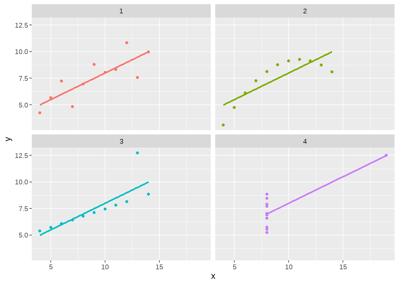
## 6 14 14 14 8 9.96 8.10 8.84 7.04实际上,这是四组(x1, y1), (x2, y2), (x3, y3), (x4, y4)。那要怎么样规整数据,
或者说怎么样把数据弄成tidy呢。这里有个技巧,你可以想象,数据能ggplot()可视化的基本上就是tidy的。
d %>%
  ggplot(aes(x = x, y = y)) +
  geom_point() +
  facet_wrap(~set)
那么,我们希望我们的数据是这样的格式
| set | x | y |
|---|---|---|
| 1 | 10 | 8.04 |
| 1 | 8 | 6.95 |
| … | ||
| 2 | 10 | 9.14 |
| 2 | 8 | 8.14 |
| … |
81.2.1 小小的回顾
我们之前讲过,数据变形中,宽表格变成长表格,
需要用到tidyr::pivot_longer()函数
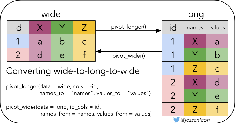
比如
## # A tibble: 2 × 5
##   id      x_1   x_2   y_1   y_2
##   <chr> <int> <int> <int> <int>
## 1 a         1     3     5     8
## 2 b         2     4     6     9
dt %>% pivot_longer(-id,
  names_to = "name",
  values_to = "vaules"
)
## # A tibble: 8 × 3
## id name vaules
## <chr> <chr> <int>
## 1 a x_1 1
## 2 a x_2 3
## 3 a y_1 5
## 4 a y_2 8
## 5 b x_1 2
## 6 b x_2 4
## 7 b y_1 6
## 8 b y_2 9有时候,我们不想要下划线后面的编号,只想保留前面的第一个字母
dt %>% pivot_longer(
  cols = -id,
  names_to = "name",
  names_pattern = "(.)_.",
  values_to = "vaules"
)
## # A tibble: 8 × 3
## id name vaules
## <chr> <chr> <int>
## 1 a x 1
## 2 a x 3
## 3 a y 5
## 4 a y 8
## 5 b x 2
## 6 b x 4
## 7 b y 6
## 8 b y 9有时候人的需求是多样的,比如不想要前面的第一个字母,只要下划线后面的编号
dt %>% pivot_longer(
  cols = -id,
  names_to = "name",
  names_pattern = "._(.)",
  values_to = "vaules"
)
## # A tibble: 8 × 3
## id name vaules
## <chr> <chr> <int>
## 1 a 1 1
## 2 a 2 3
## 3 a 1 5
## 4 a 2 8
## 5 b 1 2
## 6 b 2 4
## 7 b 1 6
## 8 b 2 9有时候我们都想要呢?
dt %>% pivot_longer(
  cols = -id,
  names_to = c("name", "group"),
  names_pattern = "(.)_(.)",
  values_to = "vaules"
)
## # A tibble: 8 × 4
## id name group vaules
## <chr> <chr> <chr> <int>
## 1 a x 1 1
## 2 a x 2 3
## 3 a y 1 5
## 4 a y 2 8
## 5 b x 1 2
## 6 b x 2 4
## 7 b y 1 6
## 8 b y 2 9有时候,我们希望"x", "y"保留在列名,那么匹配出来的第一个字母,就不能给"name",而是传给特殊的符号".value",它会收集匹配出来的字符,然后放在列名中
dt %>% pivot_longer(
  cols = -id,
  names_to = c(".value", "group"),
  names_pattern = "(.)_(.)",
  values_to = "vaules"
)
## # A tibble: 4 × 4
## id group x y
## <chr> <chr> <int> <int>
## 1 a 1 1 5
## 2 a 2 3 8
## 3 b 1 2 6
## 4 b 2 4 9是不是觉得很强大?
81.2.2 回到案例
具体来说,我们希望 x1 按照指定的正则表达式分成了两个部分 x和 1,那么1放在set下,而 x 传给了.value 当作变型后的列名.
knitr::include_graphics("images/pivot_longer_values.jpg")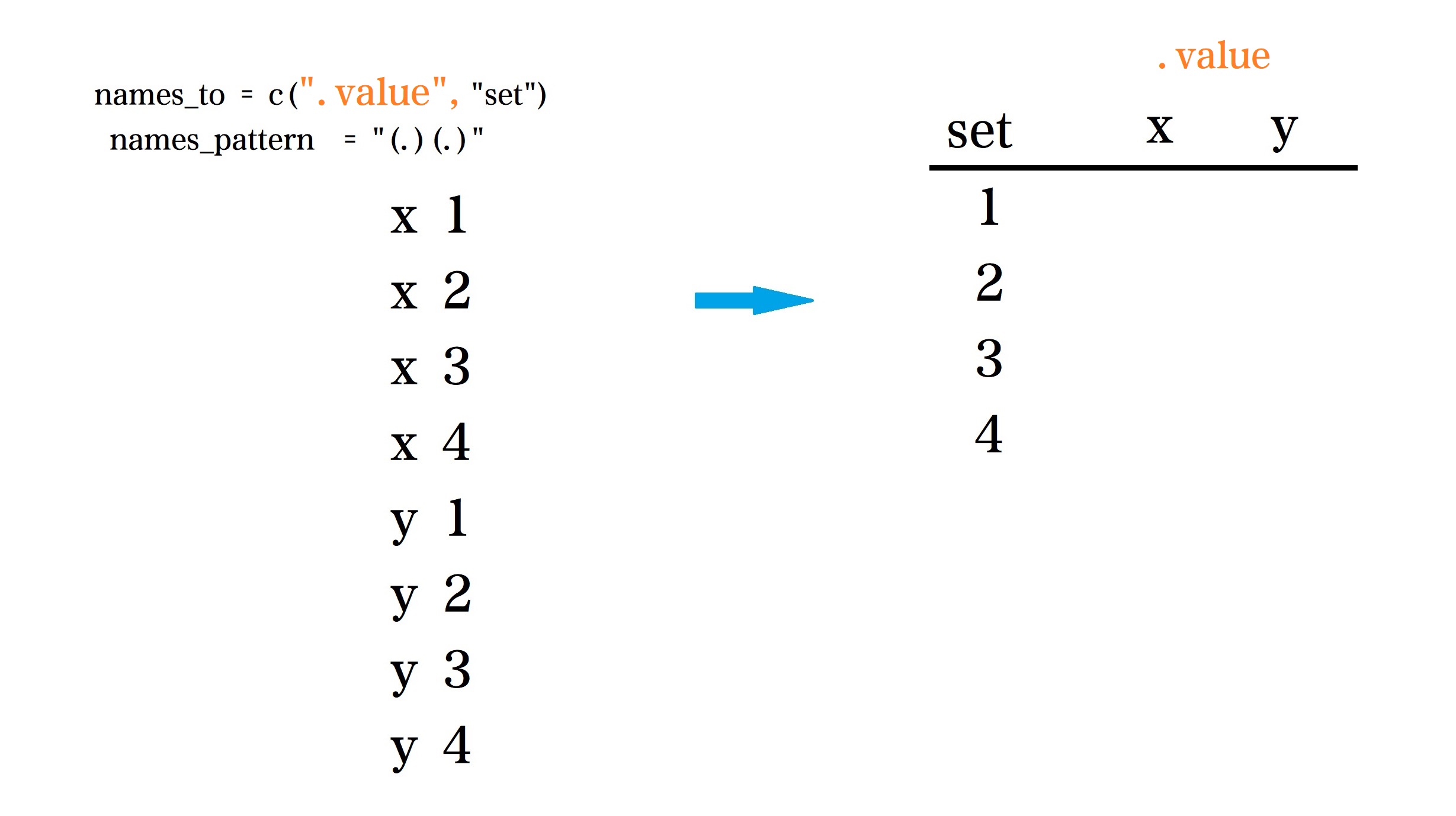
那么和上面的情况一样,使用tidyr::pivot_longer()函数
tidy_d <- d %>%
  pivot_longer(
    cols = everything(),
    names_to = c(".value", "set"),
    names_pattern = "(.)(.)"
  )
tidy_d
## # A tibble: 44 × 3
## set x y
## <chr> <dbl> <dbl>
## 1 1 10 8.04
## 2 2 10 9.14
## 3 3 10 7.46
## 4 4 8 6.58
## 5 1 8 6.95
## 6 2 8 8.14
## 7 3 8 6.77
## 8 4 8 5.76
## 9 1 13 7.58
## 10 2 13 8.74
## # ℹ 34 more rows再啰嗦下参数的含义:
-
cols = everything()表示选择所有列 -
names_to = c(".value", "set")希望变型后的列名是c(".value", "set"), 这里".value"是个特殊的符号,代表着names_pattern匹配过来的值,一般情况下,是多个值,如果传给".value"的"x, y, z",那么列名就会变成c("x", "y", "z", "set") -
names_pattern = "(.)(.)"将变换前的列名按照指定的正则表达式匹配,并且传递给names_to的对应的参数,比如这里第一个(.)传递给.value;第二个(.)传递给set.
81.3 统计
数据规整了,统计就很简单了
tidy_d_summary <- tidy_d %>%
  group_by(set) %>%
  summarise(across(
    .cols = everything(),
    .fns = lst(mean, sd, var),
    .names = "{col}_{fn}"
  ))
tidy_d_summary
## # A tibble: 4 × 7
## set x_mean x_sd x_var y_mean y_sd y_var
## <chr> <dbl> <dbl> <dbl> <dbl> <dbl> <dbl>
## 1 1 9 3.32 11 7.50 2.03 4.13
## 2 2 9 3.32 11 7.50 2.03 4.13
## 3 3 9 3.32 11 7.5 2.03 4.12
## 4 4 9 3.32 11 7.50 2.03 4.1281.4 建模
具体参考第 39 章整理的四种方法
tidy_d %>%
  group_nest(set) %>%
  mutate(
    fit = map(data, ~ lm(y ~ x, data = .x)),
    tidy = map(fit, broom::tidy),
    glance = map(fit, broom::glance)
  ) %>%
  unnest(tidy)
感觉大家更喜欢这种
## # A tibble: 8 × 6
## # Groups:   set [4]
##   set   term        estimate std.error statistic p.value
##   <chr> <chr>          <dbl>     <dbl>     <dbl>   <dbl>
## 1 1     (Intercept)    3.00      1.12       2.67 0.0257
## 2 1     x              0.500     0.118      4.24 0.00217
## 3 2     (Intercept)    3.00      1.13       2.67 0.0258
## 4 2     x              0.5       0.118      4.24 0.00218
## 5 3     (Intercept)    3.00      1.12       2.67 0.0256
## 6 3     x              0.500     0.118      4.24 0.00218
## 7 4     (Intercept)    3.00      1.12       2.67 0.0256
## 8 4 x 0.500 0.118 4.24 0.00216## # A tibble: 8 × 6
## # Groups: set [4]
## set term estimate std.error statistic p.value
## <chr> <chr> <dbl> <dbl> <dbl> <dbl>
## 1 1 (Intercept) 3.00 1.12 2.67 0.0257
## 2 1 x 0.500 0.118 4.24 0.00217
## 3 2 (Intercept) 3.00 1.13 2.67 0.0258
## 4 2 x 0.5 0.118 4.24 0.00218
## 5 3 (Intercept) 3.00 1.12 2.67 0.0256
## 6 3 x 0.500 0.118 4.24 0.00218
## 7 4 (Intercept) 3.00 1.12 2.67 0.0256
## 8 4 x 0.500 0.118 4.24 0.0021681.5 可视化看看
tidy_d %>%
  ggplot(aes(x = x, y = y, colour = set)) +
  geom_point() +
  geom_smooth(method = "lm", se = FALSE) +
  theme(legend.position = "none") +
  facet_wrap(~set)