第 69 章 贝叶斯logistic-binomial模型
library(tidyverse)
library(tidybayes)
library(rstan)

rstan_options(auto_write = TRUE)
options(mc.cores = parallel::detectCores())
theme_set(bayesplot::theme_default())
69.1 企鹅案例
筛选出物种为”Gentoo”的企鹅,并构建gender变量,male 对应1,female对应0
library(palmerpenguins)
gentoo <- penguins %>%
  filter(species == "Gentoo", !is.na(sex)) %>%
  mutate(gender = if_else(sex == "male", 1, 0))
gentoo
## # A tibble: 119 × 9
## species island bill_length_mm bill_depth_mm flipper_length_mm body_mass_g
## <fct> <fct> <dbl> <dbl> <int> <int>
## 1 Gentoo Biscoe 46.1 13.2 211 4500
## 2 Gentoo Biscoe 50 16.3 230 5700
## 3 Gentoo Biscoe 48.7 14.1 210 4450
## 4 Gentoo Biscoe 50 15.2 218 5700
## 5 Gentoo Biscoe 47.6 14.5 215 5400
## 6 Gentoo Biscoe 46.5 13.5 210 4550
## 7 Gentoo Biscoe 45.4 14.6 211 4800
## 8 Gentoo Biscoe 46.7 15.3 219 5200
## 9 Gentoo Biscoe 43.3 13.4 209 4400
## 10 Gentoo Biscoe 46.8 15.4 215 5150
## # ℹ 109 more rows
## # ℹ 3 more variables: sex <fct>, year <int>, gender <dbl>69.1.1 dotplots
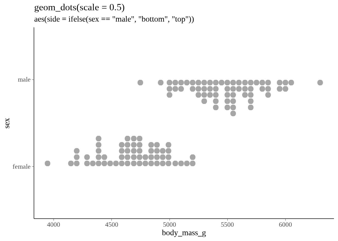
借鉴ggdist的Logit dotplots 的画法,画出dotplot
gentoo %>%
  ggplot(aes(x = body_mass_g, y = sex, side = ifelse(sex == "male", "bottom", "top"))) +
  geom_dots(scale = 0.5) +
  ggtitle(
    "geom_dots(scale = 0.5)",
    'aes(side = ifelse(sex == "male", "bottom", "top"))'
  )
\[ \begin{align*} y_i & = \text{bernoulli}( p_i) \\ p_i & =\text{logit}^{-1}(X_i \beta) \end{align*} \]
69.1.2 bayesian logit模型
stan_program <- "
data {
  int<lower=0> N;
  vector[N] x;
  int<lower=0,upper=1> y[N];
  int<lower=0> M;
  vector[M] new_x;
}
parameters {
  real alpha;
  real beta;
}
model {
  // more efficient and arithmetically stable
  y ~ bernoulli_logit(alpha + beta * x);
}
generated quantities {
  vector[M] y_epred;
  vector[M] mu = alpha + beta * new_x;

  for(i in 1:M) {
    y_epred[i] = inv_logit(mu[i]);
  }

}
"

newdata <- data.frame(
    body_mass_g = seq(min(gentoo$body_mass_g), max(gentoo$body_mass_g), length.out = 100)
   )


stan_data <- list(
  N = nrow(gentoo),
  y = gentoo$gender,
  x = gentoo$body_mass_g,
  M = nrow(newdata),
  new_x = newdata$body_mass_g
)

m <- stan(model_code = stan_program, data = stan_data)
fit <- m %>%
  tidybayes::gather_draws(y_epred[i]) %>%
  ggdist::mean_qi(.value)
fit
## # A tibble: 100 × 8
## i .variable .value .lower .upper .width .point .interval
## <int> <chr> <dbl> <dbl> <dbl> <dbl> <chr> <chr>
## 1 1 y_epred 0.0000291 0.00000000661 0.000257 0.95 mean qi
## 2 2 y_epred 0.0000351 0.00000000997 0.000307 0.95 mean qi
## 3 3 y_epred 0.0000425 0.0000000150 0.000369 0.95 mean qi
## 4 4 y_epred 0.0000515 0.0000000225 0.000446 0.95 mean qi
## 5 5 y_epred 0.0000624 0.0000000339 0.000533 0.95 mean qi
## 6 6 y_epred 0.0000757 0.0000000510 0.000643 0.95 mean qi
## 7 7 y_epred 0.0000920 0.0000000757 0.000766 0.95 mean qi
## 8 8 y_epred 0.000112 0.000000111 0.000913 0.95 mean qi
## 9 9 y_epred 0.000136 0.000000163 0.00110 0.95 mean qi
## 10 10 y_epred 0.000166 0.000000243 0.00132 0.95 mean qi
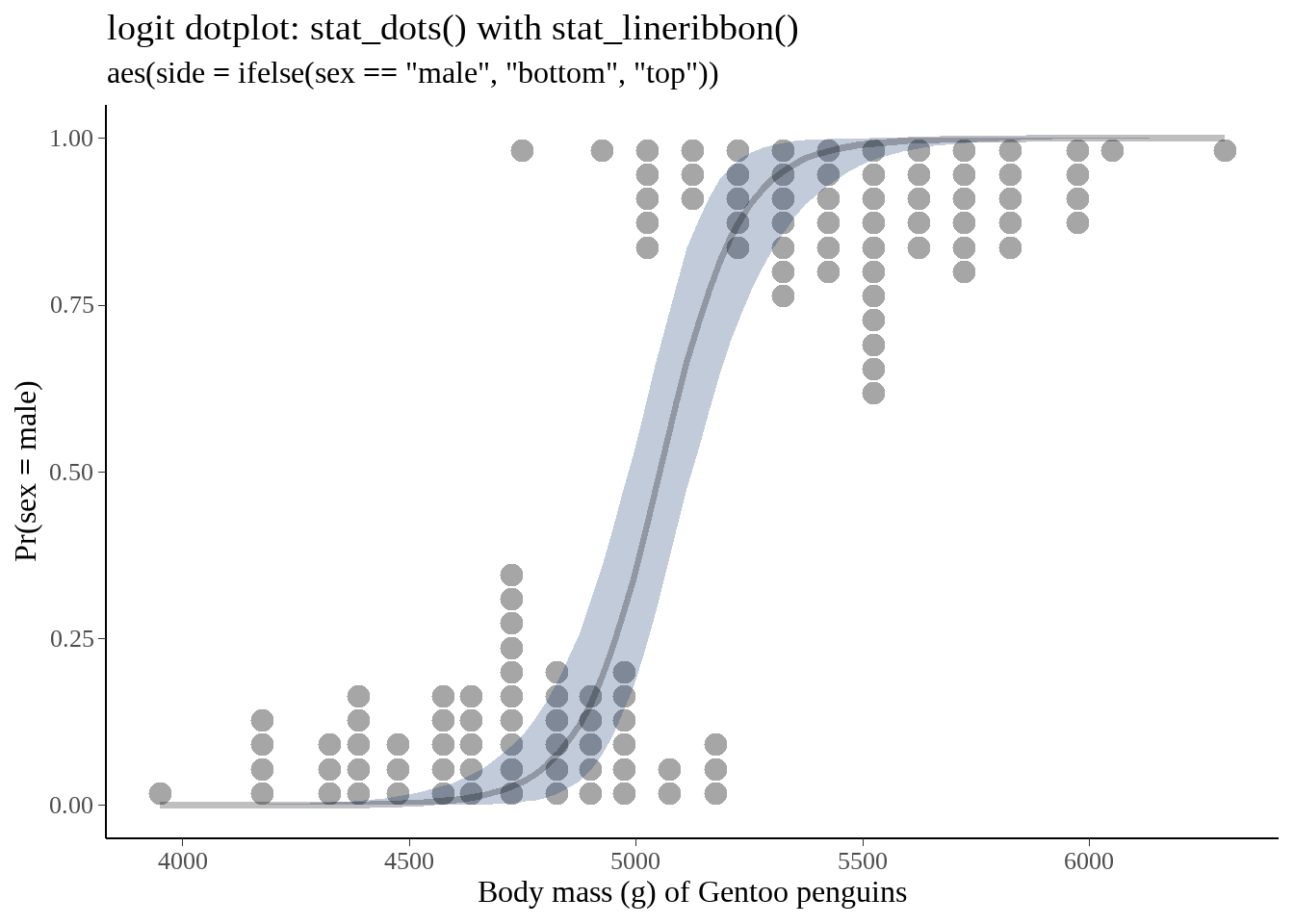
## # ℹ 90 more rows两个图画在一起
fit %>%
  bind_cols(newdata) %>%
  ggplot(aes(x = body_mass_g)) +
  geom_dots(
    data = gentoo,
    aes(y = gender, side = ifelse(sex == "male", "bottom", "top")),
    scale = 0.4
  ) +
  geom_lineribbon(
    aes(y = .value, ymin = .lower, ymax = .upper),
    alpha = 1/4,
    fill = "#08306b"
  ) +
  labs(
    title = "logit dotplot: stat_dots() with stat_lineribbon()",
    subtitle = 'aes(side = ifelse(sex == "male", "bottom", "top"))',
    x = "Body mass (g) of Gentoo penguins",
    y = "Pr(sex = male)"
  )
69.2 篮球案例
我们模拟100个选手每人投篮20次,假定命中概率是身高的线性函数,案例来源chap15.3 of [Regression and Other Stories] (page270).
n <- 100

data <-
  tibble(size   = 20,
         height = rnorm(n, mean = 72, sd = 3)) %>%
  mutate(y = rbinom(n, size = size, p = 0.4 + 0.1 * (height - 72) / 3))

head(data)
## # A tibble: 6 × 3
## size height y
## <dbl> <dbl> <int>
## 1 20 70.2 8
## 2 20 74.0 9
## 3 20 67.6 2
## 4 20 69.6 6
## 5 20 70.8 5
## 6 20 72.2 769.2.1 常规做法
##
## Call:  glm(formula = cbind(y, 20 - y) ~ height, family = binomial(link = "logit"),
##     data = data)
##
## Coefficients:
## (Intercept)       height
##    -13.6675       0.1849
##
## Degrees of Freedom: 99 Total (i.e. Null);  98 Residual
## Null Deviance:       263.6
## Residual Deviance: 137.8     AIC: 468.7
69.2.2 stan 代码
\[ \begin{align*} y_i & = \text{Binomial}(n_i, p_i) \\ p_i & =\text{logit}^{-1}(X_i \beta) \end{align*} \]
stan_program <- "
data {
  int<lower=0> N;
  int<lower=0> K;
  matrix[N, K] X;
  int<lower=0> y[N];
  int trials[N];
}
parameters {
  vector[K] beta;
}
model {

  for(i in 1:N) {
    target += binomial_logit_lpmf(y[i] | trials[i], X[i] * beta);
  }

}
"


stan_data <- data %>%
  tidybayes::compose_data(
    N      = n,
    K      = 2,
    y      = y,
    trials = size,
    X      = model.matrix(~ 1 + height)
  )

fit <- stan(model_code = stan_program, data = stan_data)
fit## Inference for Stan model: anon_model.
## 4 chains, each with iter=2000; warmup=1000; thin=1;
## post-warmup draws per chain=1000, total post-warmup draws=4000.
##
## mean se_mean sd 2.5% 25% 50% 75% 97.5% n_eff Rhat
## beta[1] -13.67 0.06 1.23 -16.17 -14.49 -13.68 -12.81 -11.35 481 1
## beta[2] 0.19 0.00 0.02 0.15 0.17 0.19 0.20 0.22 481 1
## lp__ -233.34 0.03 0.96 -235.89 -233.72 -233.04 -232.64 -232.38 775 1
##
## Samples were drawn using NUTS(diag_e) at Mon Oct 28 09:52:18 2024.
## For each parameter, n_eff is a crude measure of effective sample size,
## and Rhat is the potential scale reduction factor on split chains (at
## convergence, Rhat=1).