第 83 章 探索性数据分析-驯鹿迁移
本章我们分析加拿大哥伦比亚林地驯鹿追踪数据,数据包含了从1988年到2016年期间260只驯鹿,近250000个位置标签。
83.1 驯鹿位置跟踪
大家可以在这里了解数据集的信息,它包含了两个数据集
# devtools::install_github("thebioengineer/tidytuesdayR")
library(tidytuesdayR)

tuesdata <- tidytuesdayR::tt_load("2020-06-23")
# or
# tuesdata <- tidytuesdayR::tt_load(2020, week = 26)83.2 驯鹿的身份信息
## Rows: 286
## Columns: 14
## $ animal_id            <chr> "HR_151.510", "GR_C04", "GR_C03", "HR_151.805", "…
## $ sex                  <chr> "f", "f", "f", "f", "f", "f", "f", "f", "f", "f",…
## $ life_stage           <chr> NA, NA, NA, NA, NA, NA, NA, NA, NA, NA, NA, NA, N…
## $ pregnant             <lgl> NA, NA, NA, NA, NA, NA, NA, NA, NA, NA, NA, NA, N…
## $ with_calf            <lgl> NA, NA, NA, NA, NA, NA, NA, NA, NA, NA, NA, NA, N…
## $ death_cause          <chr> NA, NA, NA, NA, NA, NA, NA, NA, "Unknown", NA, NA…
## $ study_site           <chr> "Hart Ranges", "Graham", "Graham", "Hart Ranges",…
## $ deploy_on_longitude  <dbl> NA, NA, NA, NA, NA, NA, NA, NA, NA, NA, NA, NA, N…
## $ deploy_on_latitude   <dbl> NA, NA, NA, NA, NA, NA, NA, NA, NA, NA, NA, NA, N…
## $ deploy_on_comments   <chr> NA, NA, NA, NA, NA, NA, NA, NA, NA, NA, NA, NA, N…
## $ deploy_off_longitude <dbl> NA, NA, NA, NA, NA, NA, NA, NA, -122.6405, NA, NA…
## $ deploy_off_latitude  <dbl> NA, NA, NA, NA, NA, NA, NA, NA, 55.26054, NA, NA,…
## $ deploy_off_type      <chr> "unknown", "unknown", "unknown", "unknown", "unkn…
## $ deploy_off_comments <chr> NA, NA, NA, NA, NA, NA, NA, NA, NA, NA, NA, NA, N…## # A tibble: 260 × 2
## animal_id n
## <chr> <int>
## 1 BP_car022 1
## 2 BP_car023 1
## 3 BP_car032 1
## 4 BP_car043 1
## 5 BP_car100 1
## 6 BP_car101 1
## 7 BP_car115 1
## 8 BP_car144 1
## 9 BP_car145 1
## 10 GR_C01 2
## # ℹ 250 more rows我们发现有重复id的,怎么办?
## # A tibble: 50 × 15
##    animal_id dupe_count sex   life_stage pregnant with_calf death_cause
##    <chr>          <int> <chr> <chr>      <lgl>    <lgl>     <chr>
##  1 MO_car150          3 f     3-5        NA       FALSE     <NA>
##  2 MO_car150          3 f     3-5        NA       FALSE     <NA>
##  3 MO_car150          3 f     4-6        NA       FALSE     <NA>
##  4 QU_car137          3 f     2-3        NA       FALSE     <NA>
##  5 QU_car137          3 f     3-5        NA       FALSE     <NA>
##  6 QU_car137          3 f     3-5        NA       FALSE     <NA>
##  7 GR_C01             2 f     <NA>       NA       NA        <NA>
##  8 GR_C01             2 f     <NA>       NA       NA        <NA>
##  9 GR_C02             2 f     <NA>       NA       NA        <NA>
## 10 GR_C02             2 f     <NA>       NA       NA        <NA>
## # ℹ 40 more rows
## # ℹ 8 more variables: study_site <chr>, deploy_on_longitude <dbl>,
## #   deploy_on_latitude <dbl>, deploy_on_comments <chr>,
## #   deploy_off_longitude <dbl>, deploy_off_latitude <dbl>,
## #   deploy_off_type <chr>, deploy_off_comments <chr>
individuals %>%
  filter(deploy_on_latitude > 50) %>%
  ggplot(aes(x = deploy_on_longitude, y = deploy_on_latitude)) +
  geom_point(aes(color = study_site)) #+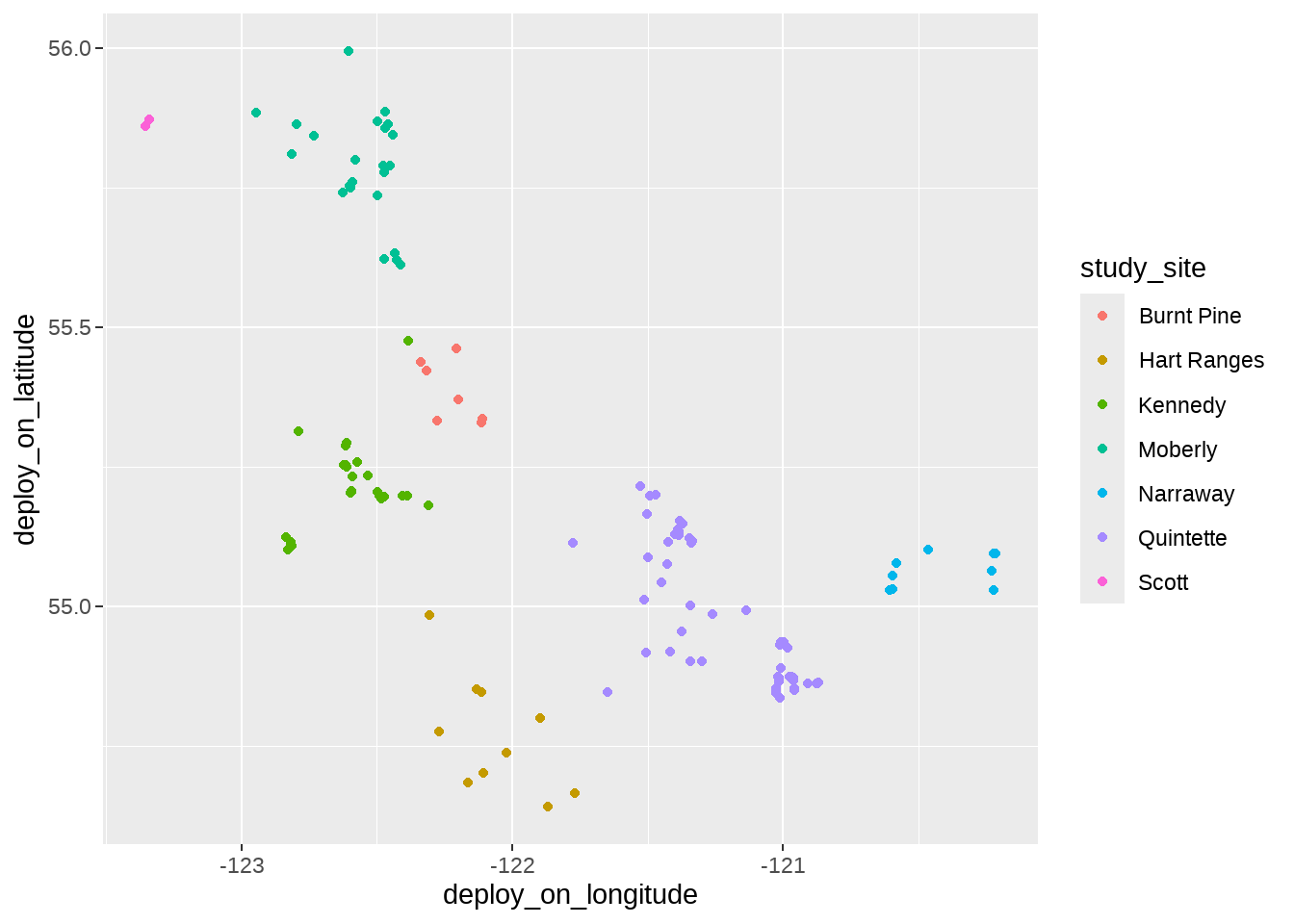
# borders("world", regions = "china")83.5 驯鹿的活动信息
简单点说,就是哪个驯鹿在什么时间出现在什么地方
locations %>%
  ggplot(aes(x = longitude, y = latitude)) +
  geom_point(aes(color = study_site))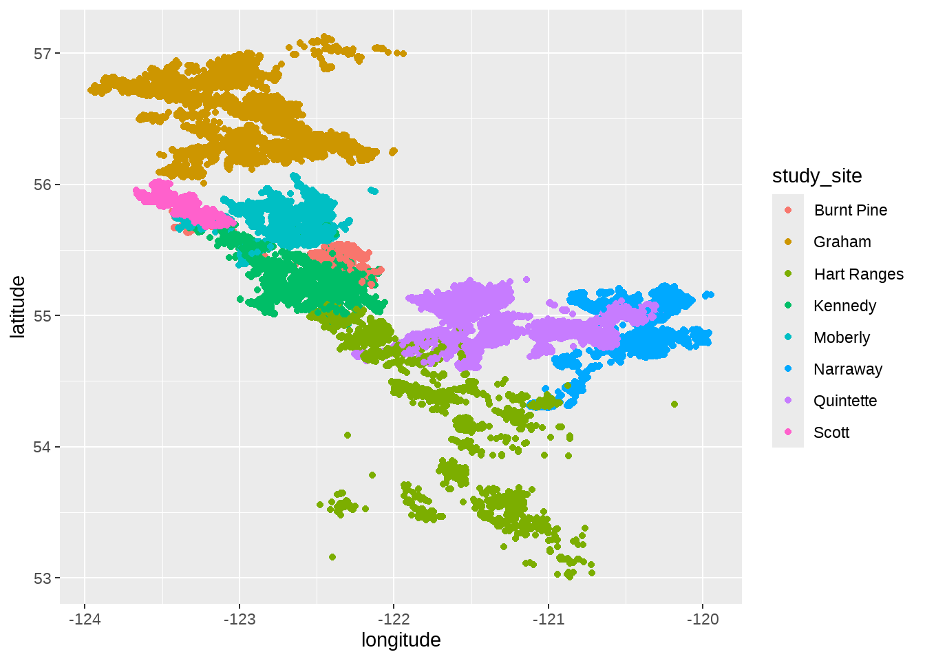
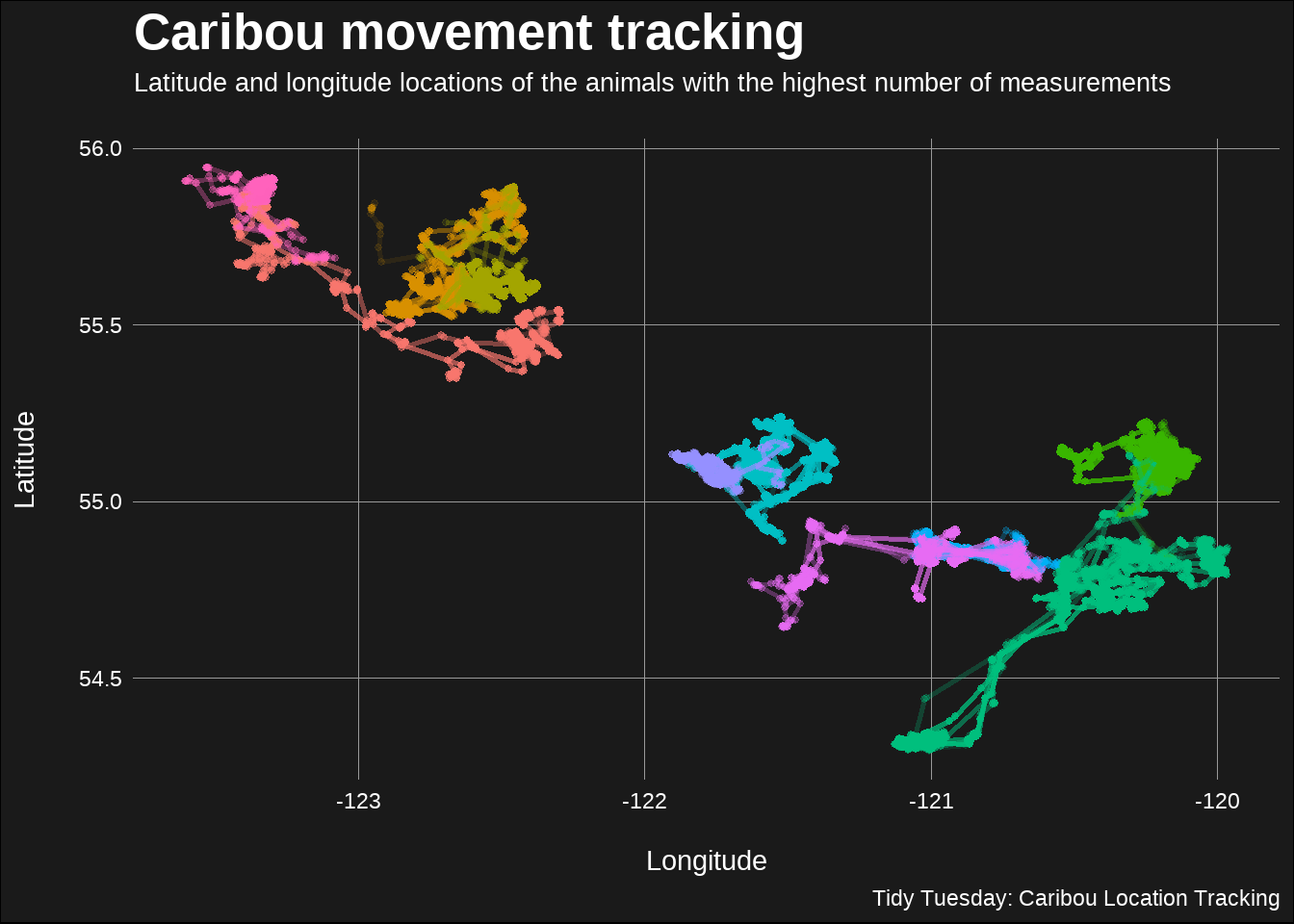
83.6 被追踪最多次的驯鹿的轨迹
top_animal_ids <-
  count(locations, animal_id, sort = TRUE) %>%
  slice(1:10) %>%
  pull(animal_id)


locations %>%
  filter(animal_id %in% top_animal_ids) %>%
  arrange(animal_id, timestamp) %>%
  group_by(animal_id) %>%
  mutate(measurement_n = row_number()) %>%
  ggplot(aes(
    x = longitude,
    y = latitude,
    color = animal_id,
    alpha = measurement_n
  )) +
  geom_point(show.legend = FALSE, size = 1) +
  geom_path(show.legend = FALSE, size = 1) +
  # scale_color_manual(values = ) +
  theme_minimal() +
  theme(
    plot.title = element_text(size = 20, face = "bold"),
    plot.subtitle = element_text(size = 10),
    text = element_text(color = "White"),
    panel.grid.minor = element_blank(),
    panel.grid.major = element_line(color = "gray60", size = 0.05),
    plot.background = element_rect(fill = "gray10"),
    axis.text = element_text(color = "white")
  ) +
  labs(
    x = "\nLongitude", y = "Latitude\n",
    title = "Caribou movement tracking",
    subtitle = "Latitude and longitude locations of the animals with the highest number of measurements\n",
    caption = "Tidy Tuesday: Caribou Location Tracking"
  )
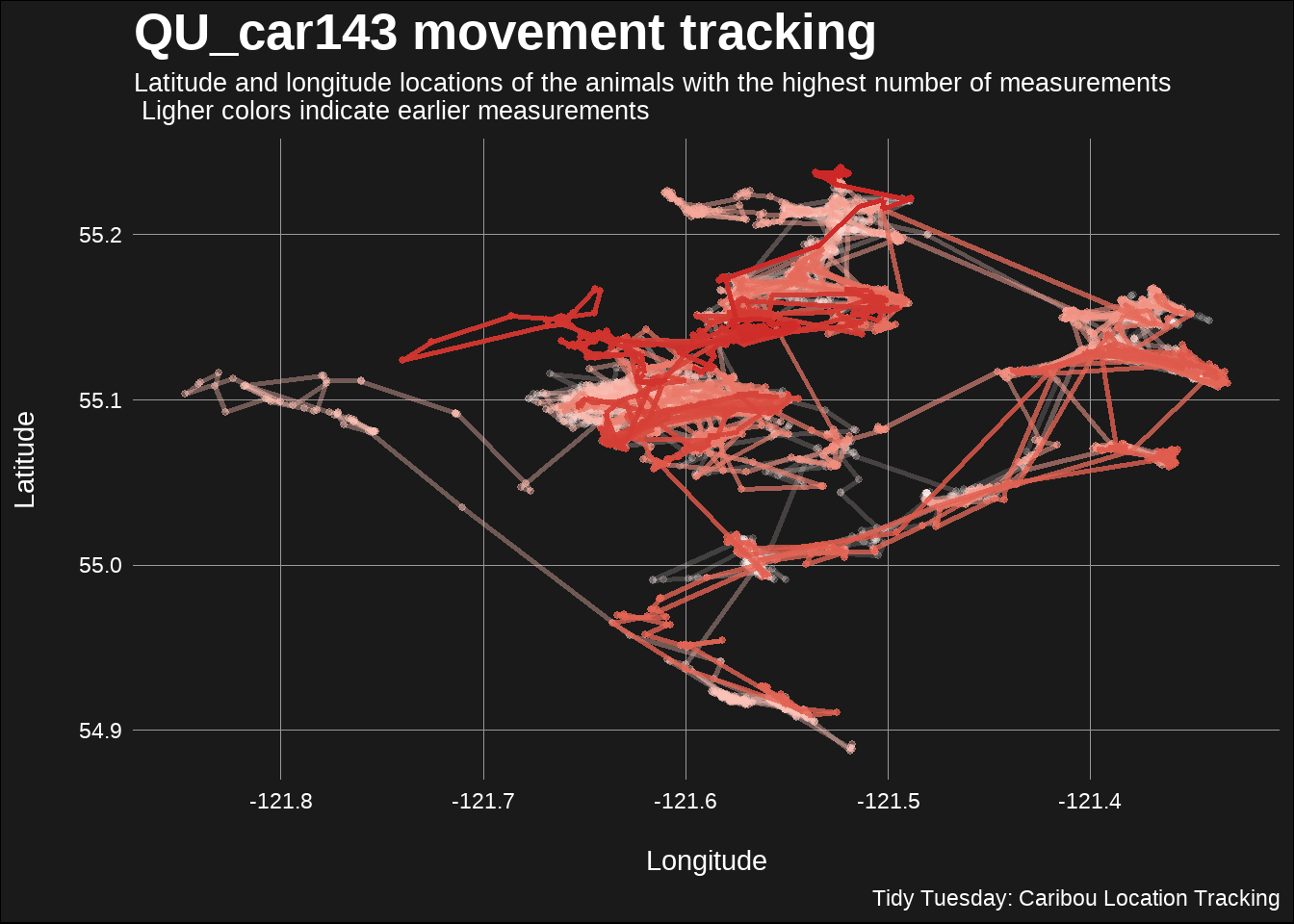
83.7 某一只驯鹿的轨迹
locations %>%
  dplyr::filter(animal_id %in% c("QU_car143")) %>%
  dplyr::arrange(animal_id, timestamp) %>%
  dplyr::group_by(animal_id) %>%
  dplyr::mutate(measurement_n = row_number()) %>%
  ggplot(aes(
    x = longitude,
    y = latitude,
    color = measurement_n,
    alpha = measurement_n
  )) +
  geom_point(show.legend = FALSE, size = 1) +
  geom_path(show.legend = FALSE, size = 1) +
  scale_color_gradient(low = "white", high = "firebrick3") +
  theme_minimal() +
  theme(
    plot.title = element_text(size = 20, face = "bold"),
    plot.subtitle = element_text(size = 10),
    text = element_text(color = "White"),
    panel.grid.minor = element_blank(),
    panel.grid.major = element_line(color = "gray60", size = 0.05),
    plot.background = element_rect(fill = "gray10"),
    axis.text = element_text(color = "white")
  ) +
  labs(
    x = "\nLongitude", y = "Latitude\n",
    title = "QU_car143 movement tracking",
    subtitle = "Latitude and longitude locations of the animals with the highest number of measurements\n Ligher colors indicate earlier measurements",
    caption = "Tidy Tuesday: Caribou Location Tracking"
  )
83.8 选择某个驯鹿,查看他的活动轨迹
example_animal <- locations %>%
  dplyr::filter(animal_id == sample(animal_id, 1)) %>%
  dplyr::arrange(timestamp)
example_animal
## # A tibble: 1,814 × 7
## event_id animal_id study_site season timestamp longitude latitude
## <dbl> <chr> <chr> <chr> <dttm> <dbl> <dbl>
## 1 2269938764 KE_car063 Kennedy Winter 2007-03-02 18:03:05 -123. 55.3
## 2 2269938765 KE_car063 Kennedy Winter 2007-03-03 14:03:04 -123. 55.3
## 3 2269938766 KE_car063 Kennedy Winter 2007-03-04 10:03:04 -123. 55.3
## 4 2269938767 KE_car063 Kennedy Winter 2007-03-05 06:03:06 -123. 55.3
## 5 2269938768 KE_car063 Kennedy Winter 2007-03-06 02:03:30 -123. 55.3
## 6 2269938769 KE_car063 Kennedy Winter 2007-03-06 22:03:06 -123. 55.3
## 7 2269938770 KE_car063 Kennedy Winter 2007-03-07 18:03:06 -123. 55.3
## 8 2269938771 KE_car063 Kennedy Winter 2007-03-08 14:03:22 -123. 55.3
## 9 2269938772 KE_car063 Kennedy Winter 2007-03-09 10:03:29 -123. 55.3
## 10 2269938773 KE_car063 Kennedy Winter 2007-03-10 06:03:05 -123. 55.3
## # ℹ 1,804 more rows
"2010-03-28 21:00:44" %>% lubridate::as_date()
"2010-03-28 21:00:44" %>% lubridate::as_datetime()
"2010-03-28 21:00:44" %>% lubridate::quarter()
example_animal %>%
  dplyr::mutate(date = lubridate::as_date(timestamp)) %>%
  ggplot(aes(x = longitude, y = latitude, color = date)) +
  geom_path()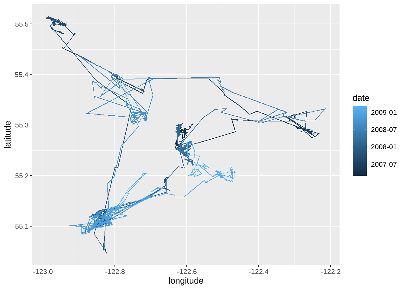
example_animal %>%
  dplyr::mutate(quarter = lubridate::quarter(timestamp) %>% as.factor()) %>%
  ggplot(aes(x = longitude, y = latitude, color = quarter)) +
  geom_path() +
  facet_wrap(vars(quarter)) +
  labs(title = "A little reindeer ran around")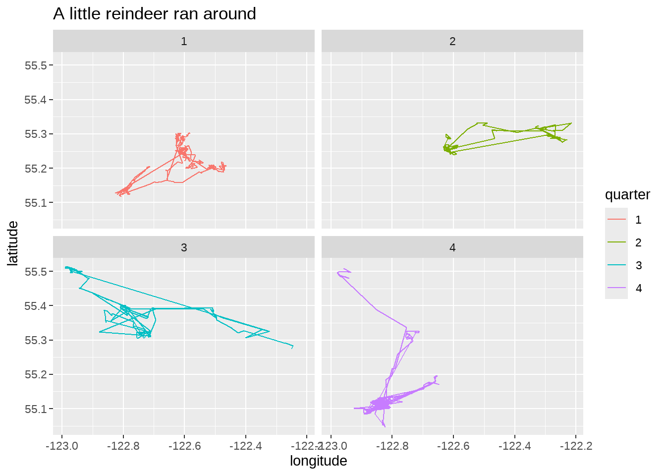
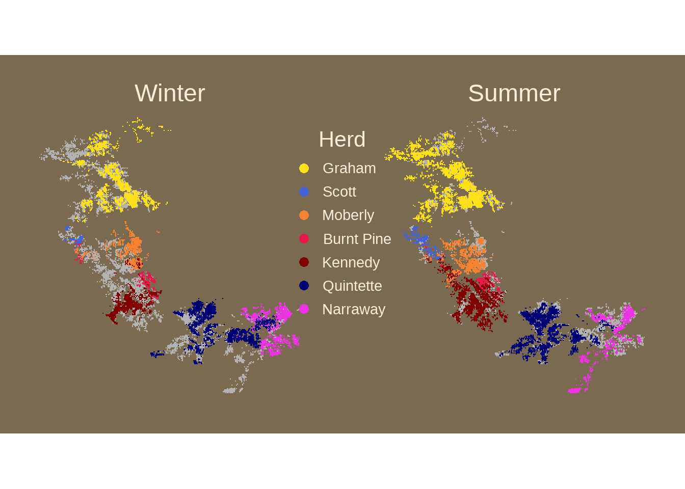
83.9 季节模式
看看驯鹿夏季和冬季运动模式,这段代码来自gkaramanis
movement <- locations %>%
  filter(study_site != "Hart Ranges") %>%
  mutate(
    season = fct_rev(season),
    longitude = round(longitude, 2),
    latitude = round(latitude, 2)
  ) %>%
  distinct(season, study_site, longitude, latitude)


ggplot(movement) +
  geom_point(aes(longitude, latitude,
    group = study_site,
    colour = study_site
  ), size = 0.1) +
  gghighlight::gghighlight(
    unhighlighted_params = list(colour = "grey70"), use_direct_label = FALSE
  ) +
  scale_colour_manual(
    values = c("#ffe119", "#4363d8", "#f58231", "#e6194B", "#800000", "#000075", "#f032e6", "#3cb44b"),
    breaks = c("Graham", "Scott", "Moberly", "Burnt Pine", "Kennedy", "Quintette", "Narraway")
  ) +
  guides(colour = guide_legend(title = "Herd", override.aes = list(size = 3))) +
  coord_fixed(ratio = 1.5) +
  facet_wrap(vars(season), ncol = 2) +
  # labs(
  #   title = "Migration patterns of Northern Caribou\nin the South Peace of British Columbia",
  #     subtitle = str_wrap("In summer, most caribou migrate towards the central core of the Rocky Mountains where they use alpine and subalpine habitat. The result of this movement to the central core of the Rocky Mountains is that some of the east side herds can overlap with west side herds during the summer.", 100),
  #     caption = str_wrap("Source: Seip DR, Price E (2019) Data from: Science update for the South Peace Northern Caribou (Rangifer tarandus caribou pop. 15) in British Columbia. Movebank Data Repository. https://doi.org/10.5441/001/1.p5bn656k | Graphic: Georgios Karamanis", 70)
  # ) +
  theme_void() +
  theme(
    legend.position = c(0.5, 0.6),
    legend.text = element_text(size = 11, colour = "#F9EED9"),
    legend.title = element_text(size = 16, hjust = 0.5, colour = "#F9EED9"),
    panel.spacing.x = unit(3, "lines"),
    plot.margin = margin(20, 20, 20, 20),
    plot.background = element_rect(fill = "#7A6A4F", colour = NA),
    strip.text = element_text(colour = "#F9EED9", size = 18),
    plot.title = element_text(colour = "white", size = 20, hjust = 0, lineheight = 1),
    plot.subtitle = element_text(colour = "white", size = 12, hjust = 0, lineheight = 1, margin = margin(10, 0, 50, 0)),
    plot.caption = element_text(colour = "grey80", size = 7, hjust = 1, margin = margin(30, 0, 10, 0))
  )
83.10 迁移速度
location_with_speed <- locations %>%
  dplyr::group_by(animal_id) %>%
  dplyr::mutate(
    last_longitude = lag(longitude),
    last_latitude = lag(latitude),
    hours = as.numeric(difftime(timestamp, lag(timestamp), units = "hours")),
    km = geosphere::distHaversine(
      cbind(longitude, latitude), cbind(last_longitude, last_latitude)
    ) / 1000,
    speed = km / hours
  ) %>%
  dplyr::ungroup()

location_with_speed
## # A tibble: 249,450 × 12
## event_id animal_id study_site season timestamp longitude latitude
## <dbl> <chr> <chr> <chr> <dttm> <dbl> <dbl>
## 1 2259197332 GR_C01 Graham Winter 2001-02-21 05:00:00 -123. 56.2
## 2 2259197333 GR_C01 Graham Winter 2001-02-21 09:00:00 -123. 56.2
## 3 2259197334 GR_C01 Graham Winter 2001-02-21 13:00:00 -123. 56.2
## 4 2259197335 GR_C01 Graham Winter 2001-02-21 17:01:00 -123. 56.2
## 5 2259197336 GR_C01 Graham Winter 2001-02-21 21:00:00 -123. 56.2
## 6 2259197337 GR_C01 Graham Winter 2001-02-22 01:00:00 -123. 56.2
## 7 2259197338 GR_C01 Graham Winter 2001-02-22 05:00:00 -123. 56.2
## 8 2259197339 GR_C01 Graham Winter 2001-02-22 09:00:00 -123. 56.2
## 9 2259197340 GR_C01 Graham Winter 2001-02-22 13:00:00 -123. 56.2
## 10 2259197341 GR_C01 Graham Winter 2001-02-22 17:00:00 -123. 56.2
## # ℹ 249,440 more rows
## # ℹ 5 more variables: last_longitude <dbl>, last_latitude <dbl>, hours <dbl>,
## # km <dbl>, speed <dbl>
location_with_speed %>%
  ggplot(aes(x = speed)) +
  geom_histogram() +
  scale_x_log10()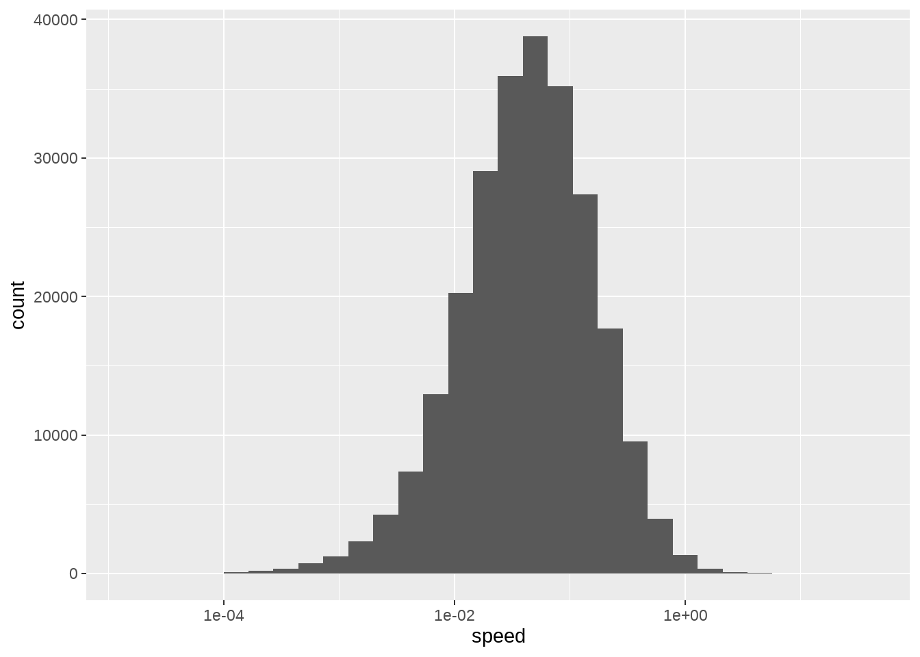
83.11 动态展示
library(gganimate)

example_animal %>%
  ggplot(aes(x = longitude, y = latitude)) +
  geom_point() +
  transition_time(time = timestamp) +
  shadow_mark(past = TRUE) +
  labs(title = "date is {frame_time}")
83.12 更多
df <- locations %>%
  dplyr::filter(
    study_site == "Graham",
    year(timestamp) == 2002
  ) %>%
  dplyr::group_by(animal_id) %>%
  dplyr::filter(
    as_date(min(timestamp)) == "2002-01-01",
    as_date(max(timestamp)) == "2002-12-31"
  ) %>%
  dplyr::ungroup() %>%
  dplyr::mutate(date = as_date(timestamp)) %>%
  dplyr::group_by(animal_id, date) %>%
  dplyr::summarise(
    longitude_centroid = mean(longitude),
    latitude_centroid = mean(latitude)
  ) %>%
  dplyr::ungroup() %>%
  tidyr::complete(animal_id, date) %>%
  dplyr::arrange(animal_id, date) %>%
  tidyr::fill(longitude_centroid, latitude_centroid, .direction = "down")
p <- df %>%
  ggplot(aes(longitude_centroid, latitude_centroid, colour = animal_id)) +
  geom_point(size = 2) +
  coord_map() +
  theme_void() +
  theme(legend.position = "none") +
  transition_time(time = date) +
  shadow_mark(alpha = 0.2, size = 0.8) +
  ggtitle("Caribou location on {frame_time}")
p