第 95 章懒人系列

R社区上很多大神，贡献了很多非常优秀的工具，节省了我们的时间，也给我们的生活增添了无限乐趣。我平时逛github的时候时整理一些，现在分享出来供像我一样的懒人用，因此本文档叫“懒人系列”。欢迎大家补充。

95.1 列名太乱了

library(tidyverse)
library(janitor)
## install.packages("janitor")
## https://github.com/sfirke/janitor

fake_raw <- tibble::tribble(
  ~id, ~`count/num`, ~W.t, ~Case, ~`time--d`, ~`%percent`,
  1L, "china", 3L, "w", 5L, 25L,
  2L, "us", 4L, "f", 6L, 34L,
  3L, "india", 5L, "q", 8L, 78L
)
fake_raw

## # A tibble: 3 × 6
##      id `count/num`   W.t Case  `time--d` `%percent`
##   <int> <chr>       <int> <chr>     <int>      <int>
## 1     1 china           3 w             5         25
## 2     2 us              4 f             6         34
## 3     3 india           5 q             8         78

fake_raw %>% janitor::clean_names()

## # A tibble: 3 × 6
##      id count_num   w_t case  time_d percent_percent
##   <int> <chr>     <int> <chr>  <int>           <int>
## 1     1 china         3 w          5              25
## 2     2 us            4 f          6              34
## 3     3 india         5 q          8              78

95.2 比count()更懂我的心

mtcars %>%
  dplyr::count(cyl, sort = TRUE) %>% 
  mutate(percent = 100 * n / sum(n))

##   cyl  n percent
## 1   8 14  43.750
## 2   4 11  34.375
## 3   6  7  21.875

mtcars %>%
  janitor::tabyl(cyl)

95.3 比distinct()更知我心

df <- tribble(
  ~id, ~date, ~store_id, ~sales,
  1, "2020-03-01", 1, 100,
  2, "2020-03-01", 2, 100,
  3, "2020-03-01", 3, 150,
  4, "2020-03-02", 1, 110,
  5, "2020-03-02", 3, 101
)

df %>%
  janitor::get_dupes(store_id)

## # A tibble: 4 × 5
##   store_id dupe_count    id date       sales
##      <dbl>      <int> <dbl> <chr>      <dbl>
## 1        1          2     1 2020-03-01   100
## 2        1          2     4 2020-03-02   110
## 3        3          2     3 2020-03-01   150
## 4        3          2     5 2020-03-02   101

df %>%
  janitor::get_dupes(date)

## # A tibble: 5 × 5
##   date       dupe_count    id store_id sales
##   <chr>           <int> <dbl>    <dbl> <dbl>
## 1 2020-03-01          3     1        1   100
## 2 2020-03-01          3     2        2   100
## 3 2020-03-01          3     3        3   150
## 4 2020-03-02          2     4        1   110
## 5 2020-03-02          2     5        3   101

95.4 代码太乱了，谁帮我整理下

## install.packages("styler")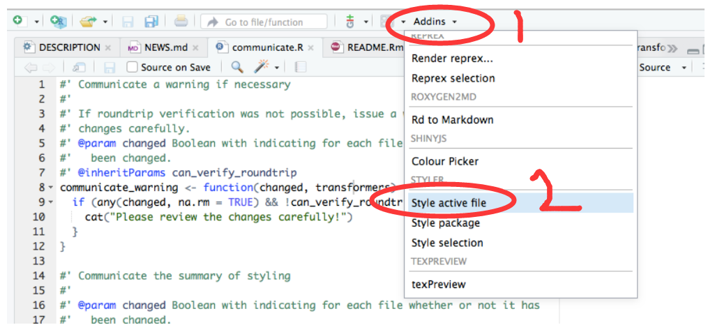

安装后，然后这两个地方点两下，就发现你的代码整齐很多了。或者直接输入

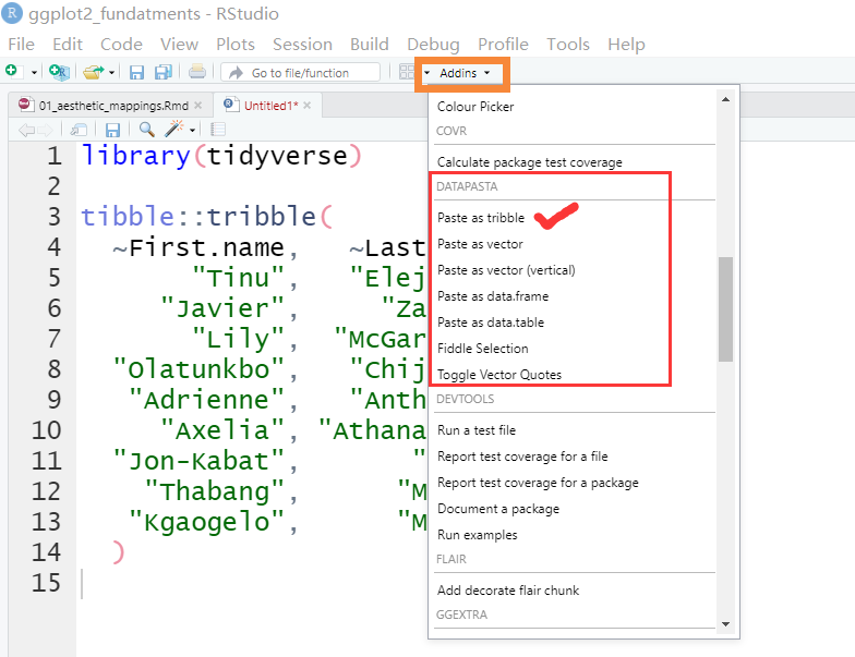
styler:::style_active_file()

95.5 用datapasta粘贴小表格

有时候想把excel或者网页上的小表格，放到R里测试下，如果用readr读取excel小数据，可能觉得麻烦，或者大材小用。比如网页https://en.wikipedia.org/wiki/Table_(information)有个表格，有偷懒的办法弄到R？

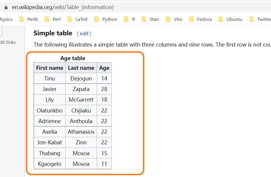
推荐一个方法

安装install.packages("datapasta")
鼠标选中并复制网页中的表格
在 Rstudio 中的Addins找到datapasta，并点击paste as tribble

95.6 谁帮我敲模型的公式

library(equatiomatic)
## https://github.com/datalorax/equatiomatic

mod1 <- lm(mpg ~ cyl + disp, mtcars)

extract_eq(mod1)

\[ \operatorname{mpg} = \alpha + \beta_{1}(\operatorname{cyl}) + \beta_{2}(\operatorname{disp}) + \epsilon \]

extract_eq(mod1, use_coefs = TRUE)

\[ \operatorname{\widehat{mpg}} = 34.66 - 1.59(\operatorname{cyl}) - 0.02(\operatorname{disp}) \]

95.7 模型有了，不知道怎么写论文？

library(report)
## https://github.com/easystats/report

model <- lm(Sepal.Length ~ Species, data = iris)
report(model)

We fitted a linear model (estimated using OLS) to predict Sepal.Length with Species (formula: Sepal.Length ~ Species). The model explains a statistically significant and substantial proportion of variance (R2 = 0.62, F(2, 147) = 119.26, p < .001, adj. R2 = 0.61). The model’s intercept, corresponding to Species = setosa, is at 5.01 (95% CI [4.86, 5.15], t(147) = 68.76, p < .001). Within this model:

The effect of Species [versicolor] is statistically significant and positive (beta = 0.93, 95% CI [0.73, 1.13], t(147) = 9.03, p < .001; Std. beta = 1.12, 95% CI [0.88, 1.37])
The effect of Species [virginica] is statistically significant and positive (beta = 1.58, 95% CI [1.38, 1.79], t(147) = 15.37, p < .001; Std. beta = 1.91, 95% CI [1.66, 2.16])

Standardized parameters were obtained by fitting the model on a standardized version of the dataset. 95% Confidence Intervals (CIs) and p-values were computed using a Wald t-distribution approximation.

95.8 模型评估一步到位

library(performance)

model <- lm(mpg ~ wt * cyl + gear, data = mtcars)
performance::check_model(model)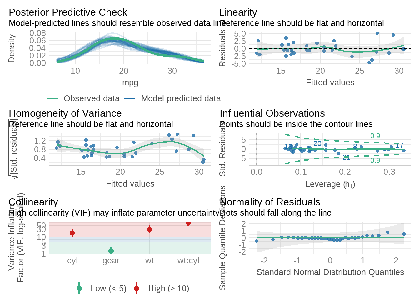

95.9 统计表格不用愁

这个确实省力不少

library(palmerpenguins)
library(gtsummary)
## https://github.com/ddsjoberg/gtsummary

penguins %>%
  drop_na() %>% 
  select(starts_with("bill_")) %>%
  tbl_summary(
    type = list(everything() ~ "continuous"),
    statistic = list(all_continuous() ~ "{mean} ({sd})")
  )

Characteristic	N = 333¹
bill_length_mm	44.0 (5.5)
bill_depth_mm	17.16 (1.97)
¹ Mean (SD)

gtsummary::trial %>%
  dplyr::select(trt, age, grade, response) %>%
  gtsummary::tbl_summary(
    by = trt,
    missing = "no"
  ) %>%
  gtsummary::add_p() %>%
  gtsummary::add_overall() %>%
  gtsummary::add_n() %>%
  gtsummary::bold_labels()

Characteristic	N	Overall N = 200¹	Drug A N = 98¹	Drug B N = 102¹	p-value²
Age	189	47 (38, 57)	46 (37, 60)	48 (39, 56)	0.7
Grade	200				0.9
I		68 (34%)	35 (36%)	33 (32%)
II		68 (34%)	32 (33%)	36 (35%)
III		64 (32%)	31 (32%)	33 (32%)
Tumor Response	193	61 (32%)	28 (29%)	33 (34%)	0.5
¹ Median (Q1, Q3); n (%)
² Wilcoxon rank sum test; Pearson’s Chi-squared test

直接复制到论文即可

t1 <-
  glm(response ~ trt + age + grade, trial, family = binomial) %>%
  gtsummary::tbl_regression(exponentiate = TRUE)

t2 <-
  survival::coxph(survival::Surv(ttdeath, death) ~ trt + grade + age, trial) %>%
  gtsummary::tbl_regression(exponentiate = TRUE)



gtsummary::tbl_merge(
  tbls = list(t1, t2),
  tab_spanner = c("**Tumor Response**", "**Time to Death**")
)

Characteristic	Tumor Response			Time to Death
Characteristic	OR¹	95% CI¹	p-value	HR¹	95% CI¹	p-value
Chemotherapy Treatment
Drug A	—	—		—	—
Drug B	1.13	0.60, 2.13	0.7	1.30	0.88, 1.92	0.2
Age	1.02	1.00, 1.04	0.10	1.01	0.99, 1.02	0.3
Grade
I	—	—		—	—
II	0.85	0.39, 1.85	0.7	1.21	0.73, 1.99	0.5
III	1.01	0.47, 2.15	>0.9	1.79	1.12, 2.86	0.014
¹ OR = Odds Ratio, CI = Confidence Interval, HR = Hazard Ratio

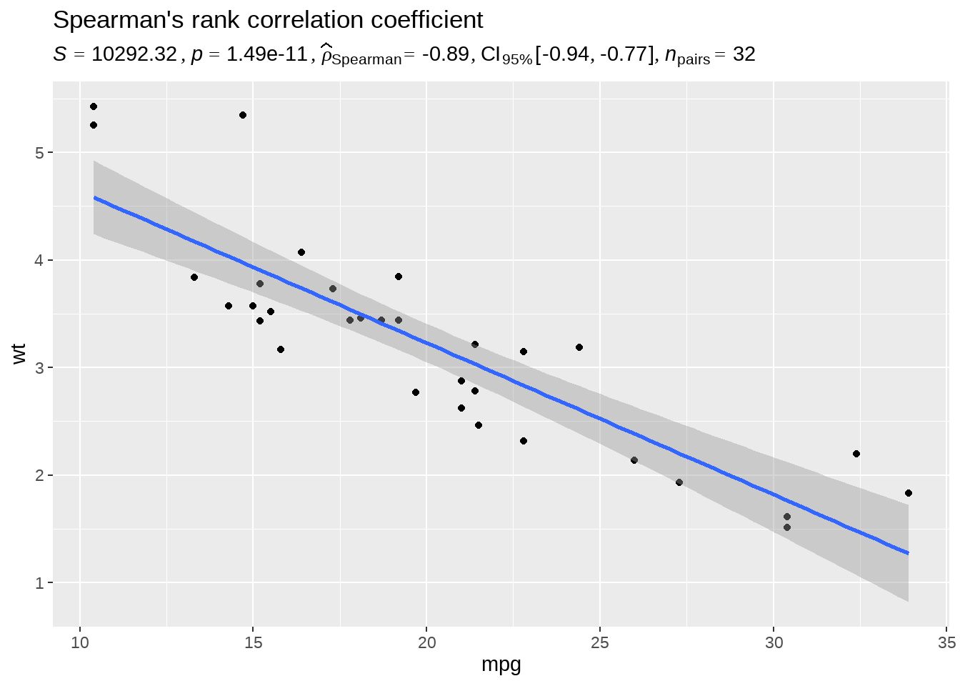
95.10 统计结果写图上

library(ggplot2)
library(statsExpressions)
# https://github.com/IndrajeetPatil/statsExpressions


# dataframe with results
results_data <- corr_test(mtcars, mpg, wt, type = "nonparametric")

# create a scatter plot
ggplot(mtcars, aes(mpg, wt)) +
  geom_point() +
  geom_smooth(method = "lm", formula = y ~ x) +
  labs(
    title = "Spearman's rank correlation coefficient",
    subtitle = parse(text = results_data$expression)
  )

95.11 正则表达式太南了

library(inferregex)
## remotes::install_github("daranzolin/inferregex")

s <- "abcd-9999-ab9"
infer_regex(s)$regex

## [1] "^[a-z]{4}-\\d{4}-[a-z]{2}\\d$"

有了它，妈妈再也不担心我的正则表达式了

95.12 颜控怎么配色？

library(ggthemr) ## devtools::install_github('cttobin/ggthemr')
ggthemr("dust")

mtcars %>%
  mutate(cyl = factor(cyl)) %>%
  ggplot(aes(x = mpg, fill = cyl, colour = cyl)) +
  geom_density(alpha = 0.75) +
  labs(fill = "Cylinders", colour = "Cylinders", x = "MPG", y = "Density") +
  legend_top()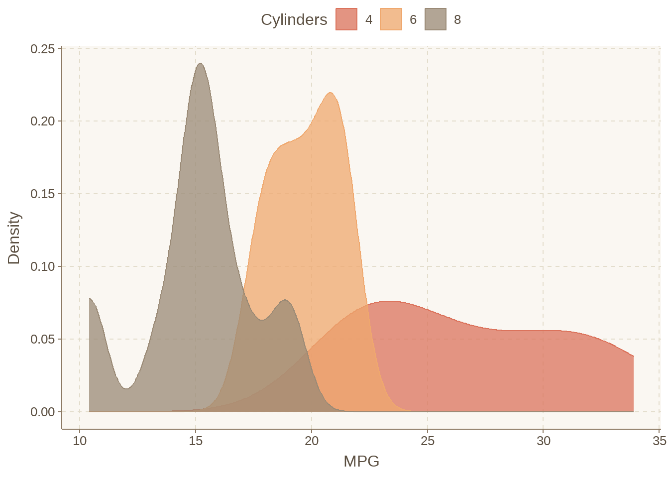

用完别忘了

ggthemr_reset()

95.13 画图颜色好看不

scales也是大神的作品，功能多多

## https://github.com/r-lib/scales
library(scales)

show_col(viridis_pal()(10))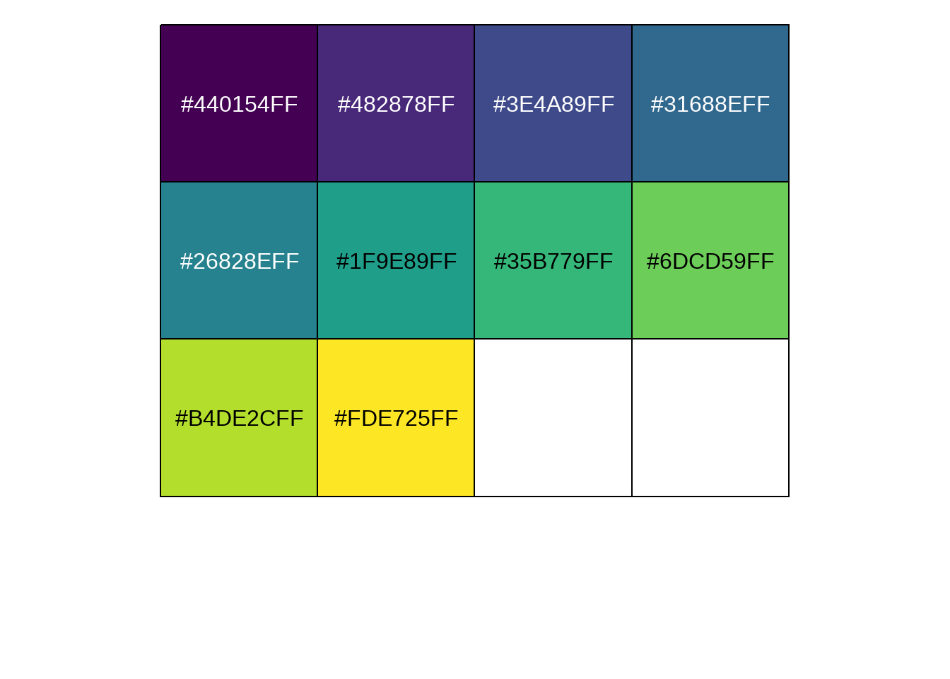

不推荐个人配色，因为我们不专业。直接用专业的配色网站 colorbrewer

先看看颜色，再选择

95.14 宏包太多

library(pacman)
## p_load(lattice, foreign, boot, rpart)

唉，这个library()都要偷懒，真服了你们了

95.15 犹抱琵琶半遮面

## https://github.com/EmilHvitfeldt/gganonymize
library(ggplot2)
library(gganonymize)

ggg <-
  ggplot(mtcars, aes(as.factor(cyl))) +
  geom_bar() +
  labs(
    title = "Test title",
    subtitle = "Test subtitle, this one have a lot lot lot lot lot more text then the rest",
    caption = "Test caption",
    tag = 1
  ) +
  facet_wrap(~vs)

gganonomize(ggg)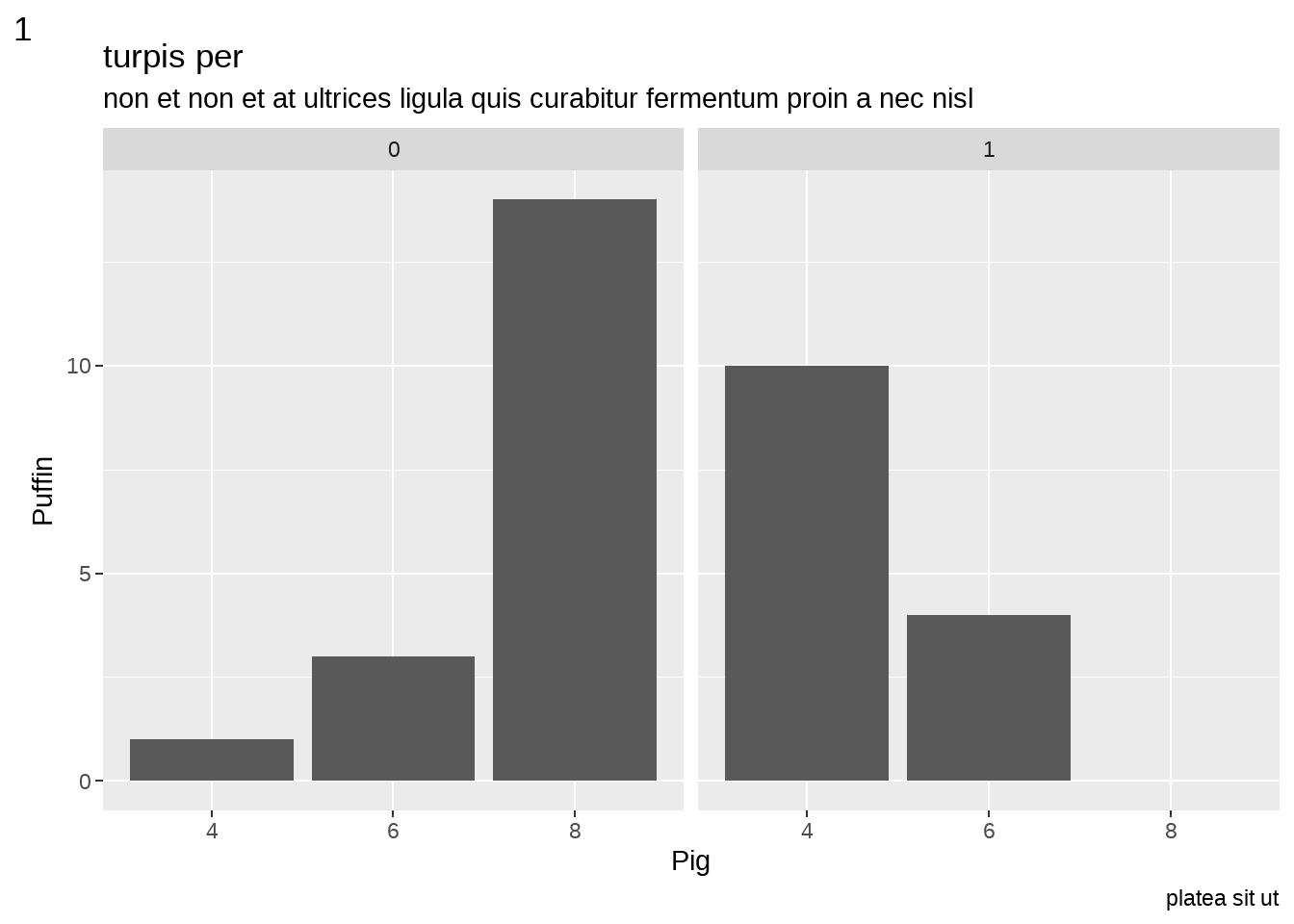

你可以看我的图，但就不想告诉你图什么意思，因为我加密了

95.16 整理Rmarkdown

# remotes::install_github("tjmahr/WrapRmd")
# remotes::install_github("fkeck/quickview")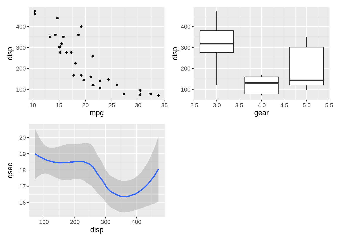
# remotes::install_github("mwip/beautifyR")

95.17 如何有效的提问

直接看官方网站，这里不举例了

## install.packages("reprex")
## https://reprex.tidyverse.org/

95.18 程序结束后记得提醒我

## beepr::beep(sound = "mario")

你听到了声音吗?

95.19 多张图摆放

library(patchwork)
p1 <- ggplot(mtcars) +
  geom_point(aes(mpg, disp))

p2 <- ggplot(mtcars) +
  geom_boxplot(aes(gear, disp, group = gear))

p3 <- ggplot(mtcars) +
  geom_smooth(aes(disp, qsec))

# Side by side
p1 + p2 + p3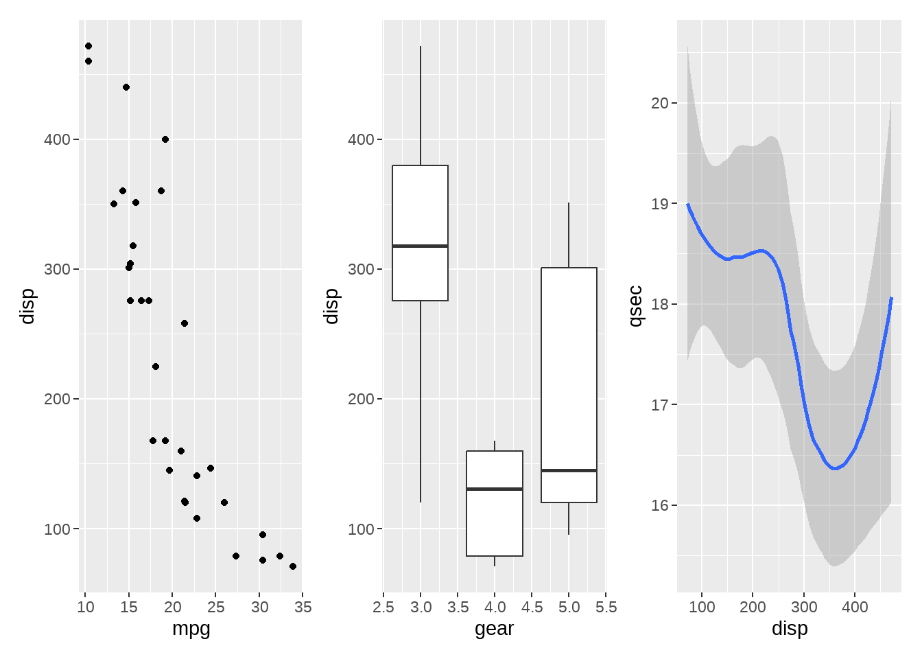

# On top of each other
p1 / p2 / p3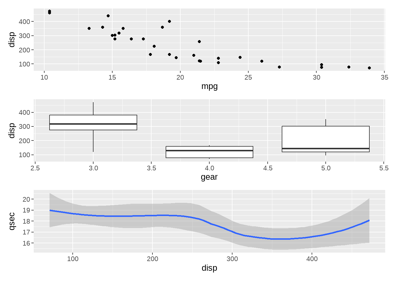

# Grid
p1 / (p2 + p3)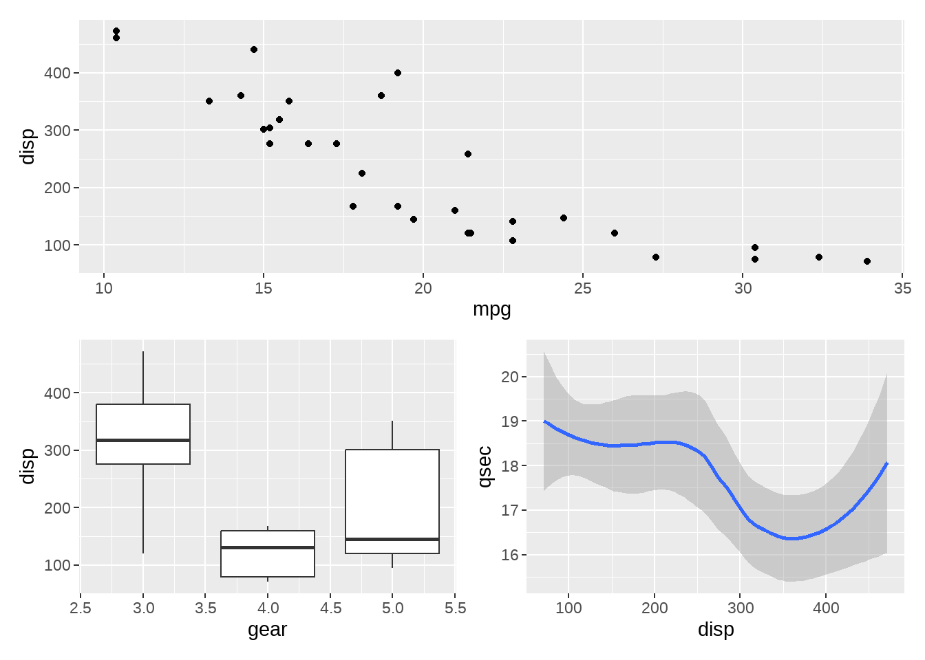

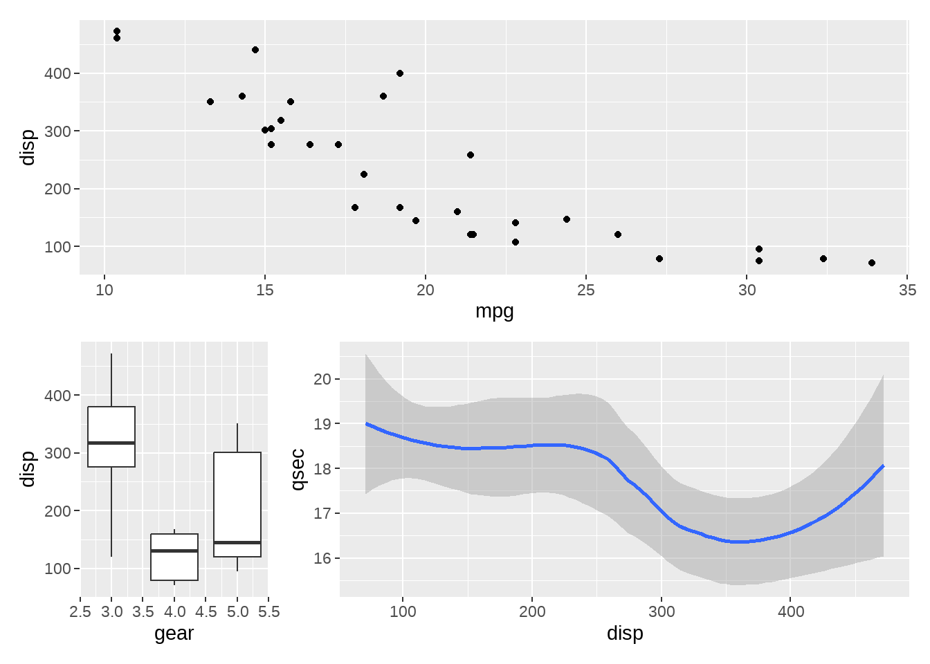
# plot_layout()

p1 + p2 + p3 +
  plot_layout(
    nrow = 2,
    ncol = 2
  )

# layout

layout <- "
AAAA
BCCC
"

p1 + p2 + p3 +
  plot_layout(
    design = layout
  )

95.20 缺失值处理

library(naniar)
## https://github.com/njtierney/naniar

airquality %>%
  group_by(Month) %>%
  naniar::miss_var_summary()

## # A tibble: 25 × 4
## # Groups:   Month [5]
##    Month variable n_miss pct_miss
##    <int> <chr>     <int>    <num>
##  1     5 Ozone         5     16.1
##  2     5 Solar.R       4     12.9
##  3     5 Wind          0      0  
##  4     5 Temp          0      0  
##  5     5 Day           0      0  
##  6     6 Ozone        21     70  
##  7     6 Solar.R       0      0  
##  8     6 Wind          0      0  
##  9     6 Temp          0      0  
## 10     6 Day           0      0  
## # ℹ 15 more rows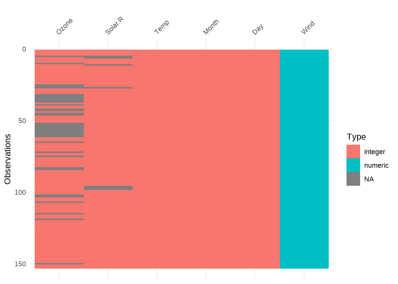

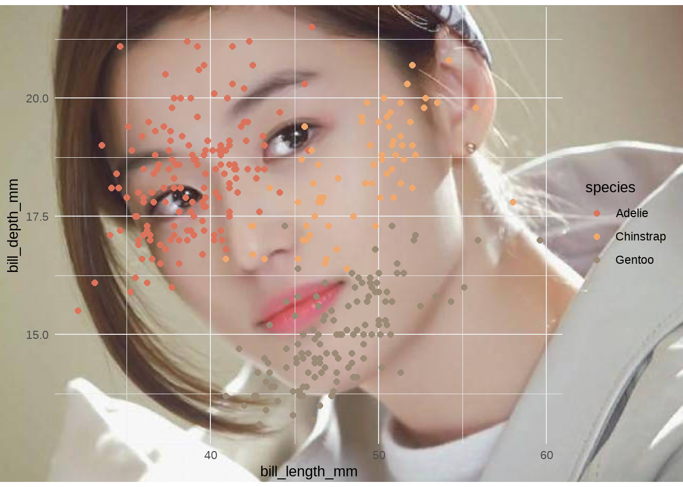
95.21 看看数据什么情况

library(visdat)

vis_dat(airquality)

95.22 让妹纸激发你的热情

library(tidyverse)
library(cowplot)

plot <- penguins %>% 
  ggplot(aes(x = bill_length_mm, y = bill_depth_mm)) +
  geom_point(aes(colour = species), size = 2) +
  theme_minimal()


ggdraw() + 
  draw_image("./images/mm.jpeg") + 
  draw_plot(plot)

95.23 管道都不想

管道都不想写，写代码还有美感？

## library(nakepipe)

95.24 各种插件，任君选取

## https://github.com/daattali/addinslist

94 tidyverse中行方向的操作

96 Pandas vs. dplyr谁是数据分析中最好用的宏包

第 95 章 懒人系列